Introduction

Most statistical learning models require that predictors take numeric form. Therefore, when a researcher wishes to include a categorical variable with more than two levels in a multiple regression prediction model, additional steps are needed to insure that the results are interpretable. There are a variety of coding systems that can be used when recoding categorical variables.

The most common is referred to as one-hot encoding, where categorical variables are transposed so that each level of the feature is represented as a boolean value. In this method, each category is mapped to a vector that contains 1 and 0 denoting the presence or absence of the feature. The number of vectors depends on the number of feature categories. Label encoding is a pure numeric conversion of the levels of a categorical variable. Caution should be used with label encoding unordered categorical variables because most models will treat them as ordered numeric features. If a categorical feature is naturally ordered then label encoding is a natural choice (most commonly referred to as ordinal encoding). Target encoding is the process of replacing a categorical value with the mean (regression) or proportion (classification) of the target variable. Target encoding runs the risk of data leakage since you are using the response variable to encode a feature.

Because one-hot encoding is one of the most popular encoding methods, we will explore its use in linear regression. One-hot encoding adds new features to a dataset and thus can significantly increase the dimensionality of the data. For those datasets with many categorical variables and where the categorical variables in turn have many unique levels, the number of features can quickly escalate. In these cases, label/ordinal encoding or some other alternative should be explored.

Data

Let’s use the kaggle craft beers dataset ( https://www.kaggle.com/nickhould/craft-cans). This dataset was collected in January 2017 and contains a list of 2,410 US craft beers and 510 US breweries. The dataset consists of two comma-delimited files, beers.csv and breweries.csv, that are linked together by an “id” variable.

The primary numeric variables are ABV and IBU. ABV stands for alcohol by volume, a measurement of the alcohol content in terms of the percentage volume of alcohol per volume of beer. Each style of beer has a certain ABV range, typically varying from less than 3.2 percent to greater than 14 percent. IBU is an abbreviation for the International Bitterness Units scale, a gauge of the bitterness of a beer. IBUs measure the parts-per-million of isohumulone, the acid found in hops that gives beer its bitter taste. Though the IBU scale can be used as a general guideline for taste, with lower IBUs corresponding to less bitterness and vice versa, it’s important to note that malt and other flavors can mask the taste of bitterness in beer.

Let’s load the two dataset files.

# Load libraries
library(tidyverse)
library(readr)
library(purrr)
library(ggthemes)
library(caret)
library(vtreat)

# Load data
beers <- read_csv('./data/beers.csv')
breweries <- read_csv('./data/breweries.csv')

Let’s first inspect the structure of the beers data.

glimpse(beers)

## Rows: 2,410
## Columns: 8
## $ X1         <dbl> 0, 1, 2, 3, 4, 5, 6, 7, 8, 9, 10, 11, 12, 13, 14, 15, 16, 1~
## $ abv        <dbl> 0.050, 0.066, 0.071, 0.090, 0.075, 0.077, 0.045, 0.065, 0.0~
## $ ibu        <dbl> NA, NA, NA, NA, NA, NA, NA, NA, NA, NA, NA, NA, NA, NA, 60,~
## $ id         <dbl> 1436, 2265, 2264, 2263, 2262, 2261, 2260, 2259, 2258, 2131,~
## $ name       <chr> "Pub Beer", "Devil's Cup", "Rise of the Phoenix", "Sinister~
## $ style      <chr> "American Pale Lager", "American Pale Ale (APA)", "American~
## $ brewery_id <dbl> 408, 177, 177, 177, 177, 177, 177, 177, 177, 177, 177, 177,~
## $ ounces     <dbl> 12.0, 12.0, 12.0, 12.0, 12.0, 12.0, 12.0, 12.0, 12.0, 12.0,~

DataExplorer::plot_missing(beers)

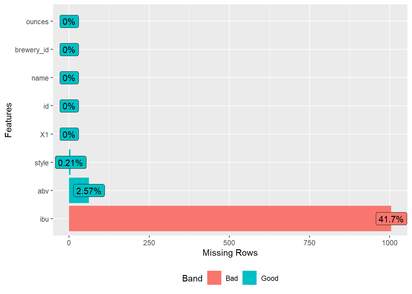
The beers data consists of 8 variables with 2,410 observations. Almost 42 percent of the ibu measurements are missing. Now, let’s inspect the structure of the breweries data.

glimpse(breweries)

## Rows: 558
## Columns: 4
## $ X1    <dbl> 0, 1, 2, 3, 4, 5, 6, 7, 8, 9, 10, 11, 12, 13, 14, 15, 16, 17, 18~
## $ name  <chr> "NorthGate Brewing", "Against the Grain Brewery", "Jack's Abby C~
## $ city  <chr> "Minneapolis", "Louisville", "Framingham", "San Diego", "San Fra~
## $ state <chr> "MN", "KY", "MA", "CA", "CA", "SC", "CO", "MI", "MI", "MI", "MI"~

DataExplorer::plot_missing(breweries)

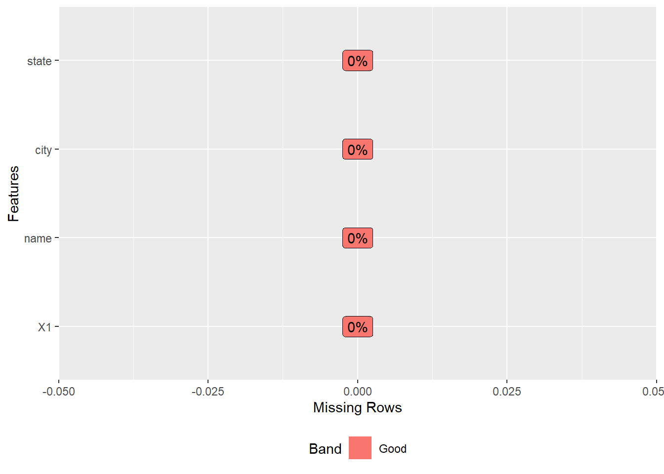
The breweries data consists of 4 variables with 558 observations and no missing values.

Data Processing

Let’s join the two data files. In the previous section we saw that all rows of beers have a brewery_id. During the joining operation, let’s conduct some minor cleaning of the final dataset.

beers_breweries <- beers %>%
  dplyr::select(-X1, -id) %>% 
  left_join(breweries, by = c('brewery_id' = 'X1')) %>%
  mutate(abv = abv * 100) %>%
  rename(beer = name.x, brewery = name.y)

Let’s view the final, joined dataset.

glimpse(beers_breweries)

## Rows: 2,410
## Columns: 9
## $ abv        <dbl> 5.0, 6.6, 7.1, 9.0, 7.5, 7.7, 4.5, 6.5, 5.5, 8.6, 7.2, 7.3,~
## $ ibu        <dbl> NA, NA, NA, NA, NA, NA, NA, NA, NA, NA, NA, NA, NA, NA, 60,~
## $ beer       <chr> "Pub Beer", "Devil's Cup", "Rise of the Phoenix", "Sinister~
## $ style      <chr> "American Pale Lager", "American Pale Ale (APA)", "American~
## $ brewery_id <dbl> 408, 177, 177, 177, 177, 177, 177, 177, 177, 177, 177, 177,~
## $ ounces     <dbl> 12.0, 12.0, 12.0, 12.0, 12.0, 12.0, 12.0, 12.0, 12.0, 12.0,~
## $ brewery    <chr> "10 Barrel Brewing Company", "18th Street Brewery", "18th S~
## $ city       <chr> "Bend", "Gary", "Gary", "Gary", "Gary", "Gary", "Gary", "Ga~
## $ state      <chr> "OR", "IN", "IN", "IN", "IN", "IN", "IN", "IN", "IN", "IN",~

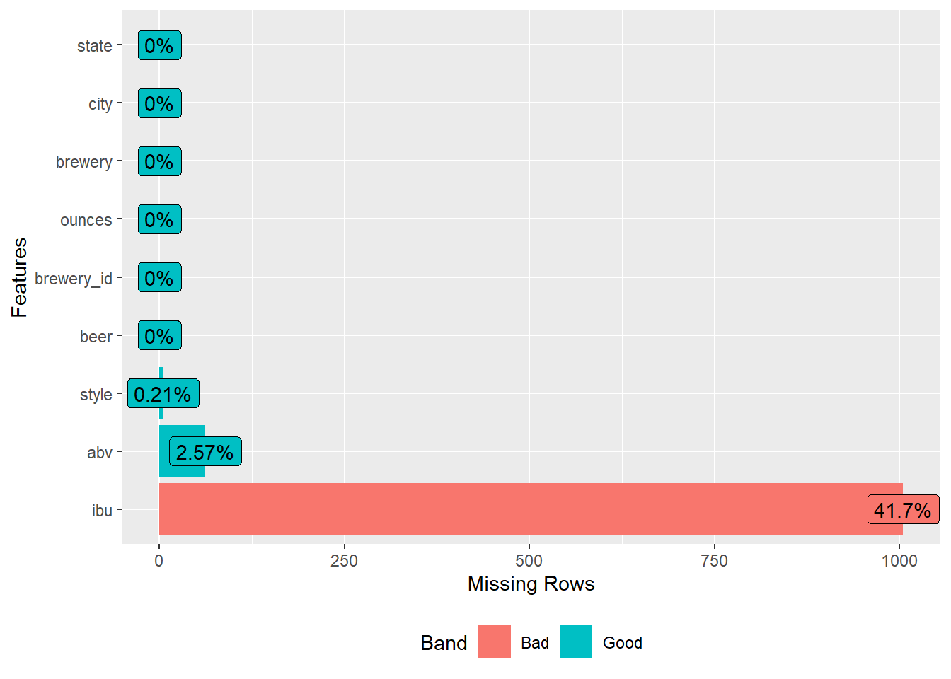
DataExplorer::plot_missing(beers_breweries)

Inspect Data

Let’s evaulate which state had the most craft breweries. Recall this dataset was complied in January 2017 and likely does not reflect the current craft beer market.

First, let’s get the top 20 states with the most craft breweries in 2017.

top_20_states <- breweries %>% 
  group_by(state) %>%
  summarise(n_breweries = n()) %>%
  arrange(desc(n_breweries)) %>%
  top_n(20)

Now, let’s calculate the average number of craft breweries by state in 2017.

avg_breweries <- breweries %>%
  group_by(state) %>% 
  summarise(n = n()) %>%
  summarise(mean = mean(n)) %>%
  '$'(mean)

Finally, let’s plot the data.

ggplot(data = top_20_states,
       aes(x = reorder(state, -n_breweries), y = n_breweries)) +
  geom_col( fill = '#4B77BE') + 
  geom_hline(yintercept = avg_breweries, color = '#DC3023',
             linetype = 2, size = 1) +
  theme_minimal() + 
  labs(title = 'Number of craft beer breweries by state',
       x = 'State',
       y = 'Number of breweries') +
  theme(axis.text.x = element_text(angle = 90, hjust = 0.5, vjust = 0.5))

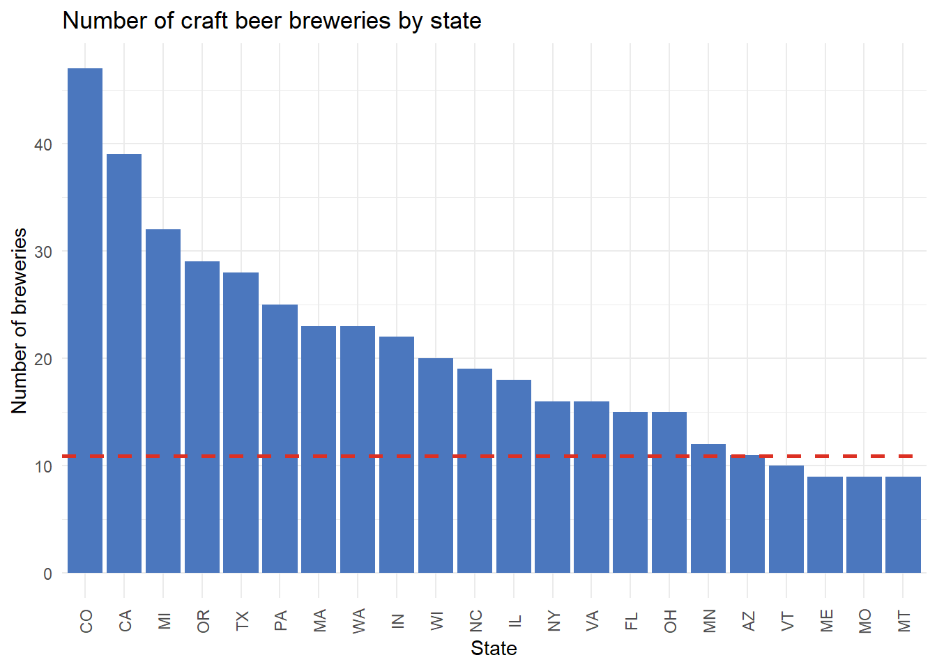
Colorado had 47 craft breweries in 2017, which is the most in our dataset. Maine, Missouri, and Montana had 9 craft breweries each and thus that accouts for the two additional states listed in our top 20. The average number of craft breweries across all states was approximately 11.

We can also inspect which cities had the most craft breweries in 2017.

# Top 20 cities
cities_count <- breweries %>% 
  group_by(city) %>%
  summarise(n_breweries = n()) %>%
  arrange(desc(n_breweries)) %>%
  top_n(20)

# Calculate average number of breweries by city
avg_breweries_city <- breweries %>%
  group_by(city) %>% 
  summarise(n = n()) %>% 
  summarise(mean = mean(n)) %>%
  '$'(mean)

ggplot(data = cities_count,
       aes(x = reorder(city, -n_breweries), y = n_breweries)) +
  geom_col(fill = '#03A678') + 
  geom_hline(yintercept = avg_breweries_city,
             color = '#FFA400', size = 1) +
  theme_minimal() + 
  labs(title = 'Number of craft beer breweries by City',
       x = 'City',
       y = 'Number of breweries') +
  theme(axis.text.x = element_text(angle = 90, hjust = 0.5, vjust = 0.5))

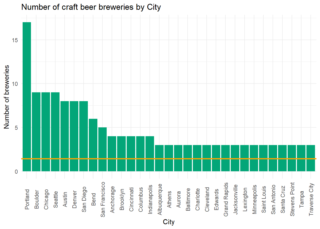
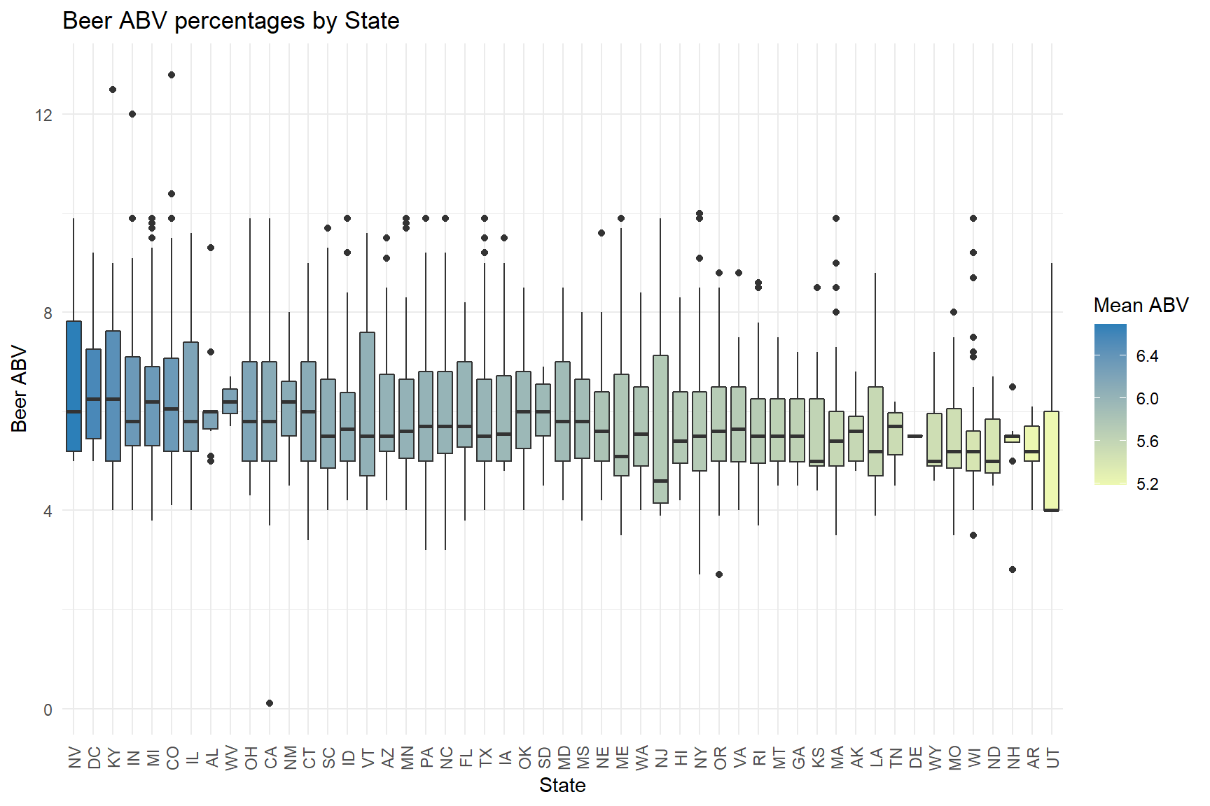
Portland had 17 craft breweries in 2017, the most in our dataset. The type and stye of beer varies across the US, so let’s look to see which cities on average have the highest and lowest ABV beers.

beers_breweries %>%
  group_by(state) %>%
  mutate(mean_abv = mean(abv, na.rm = T)) %>%
  ggplot(aes(x = reorder(state, -mean_abv), y = abv, fill = mean_abv)) +
    geom_boxplot() +
    scale_y_continuous(breaks = seq(0,12, 4)) +
    labs(title = 'Beer ABV percentages by State',
         x = 'State',
         y = 'Beer ABV') +
    scale_fill_continuous(low = '#edf8b1',
                          high = '#2c7fb8',
                          name = 'Mean ABV') +
    theme_minimal() + 
    theme(axis.text.x = element_text(angle = 90, hjust = 0.5, vjust = 0.5))

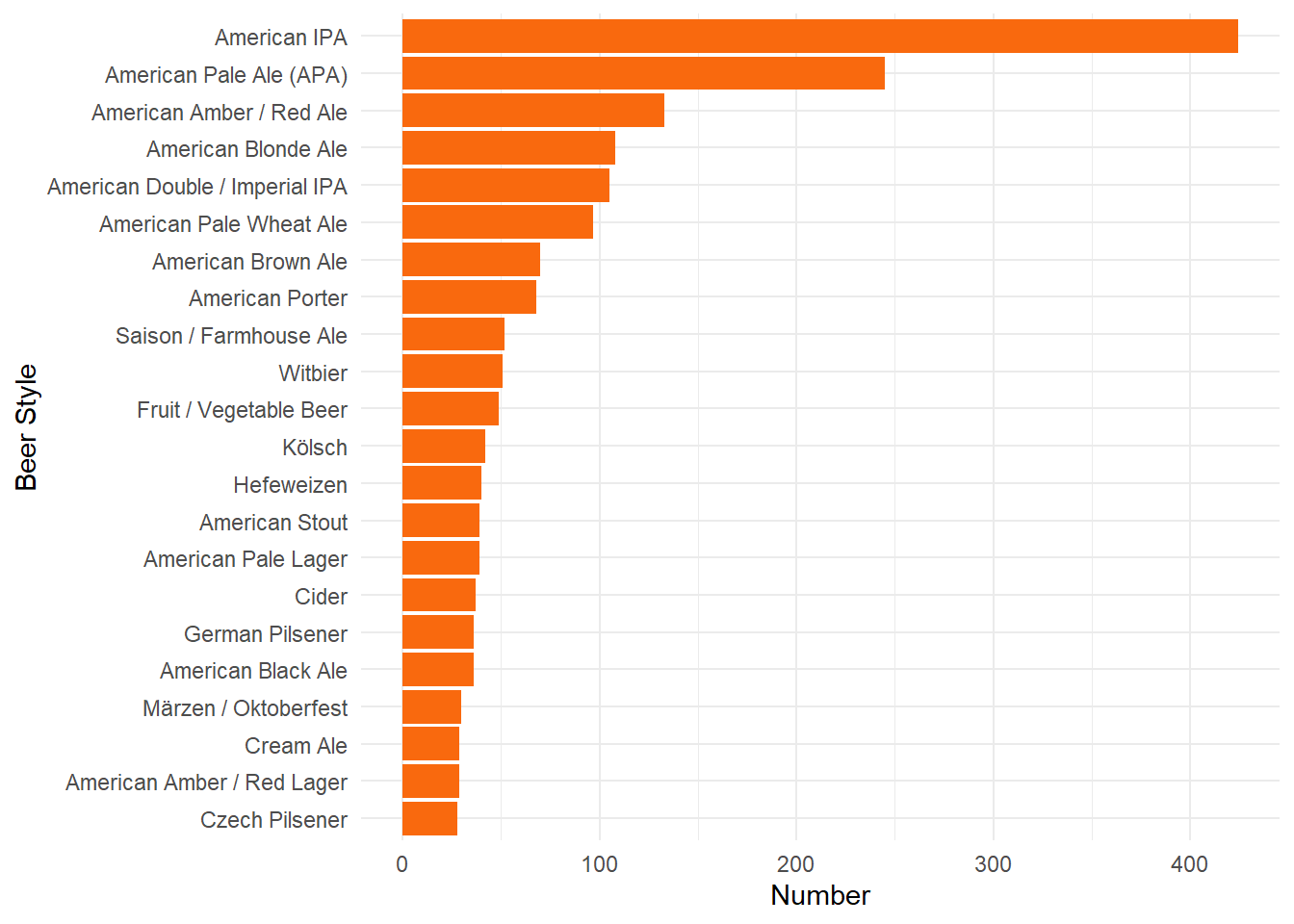
Let’s see what stylies of craft beer were the most popular were in 2017.

beers_breweries %>% 
  group_by(style) %>%
  summarise(count = n()) %>%
  filter(count > 25) %>%
  ggplot(aes(reorder(style, count), count)) +
  geom_col(fill = '#F9690E') +
  labs(x = 'Beer Style',
       y = 'Number') +
  theme_minimal() + 
  coord_flip()

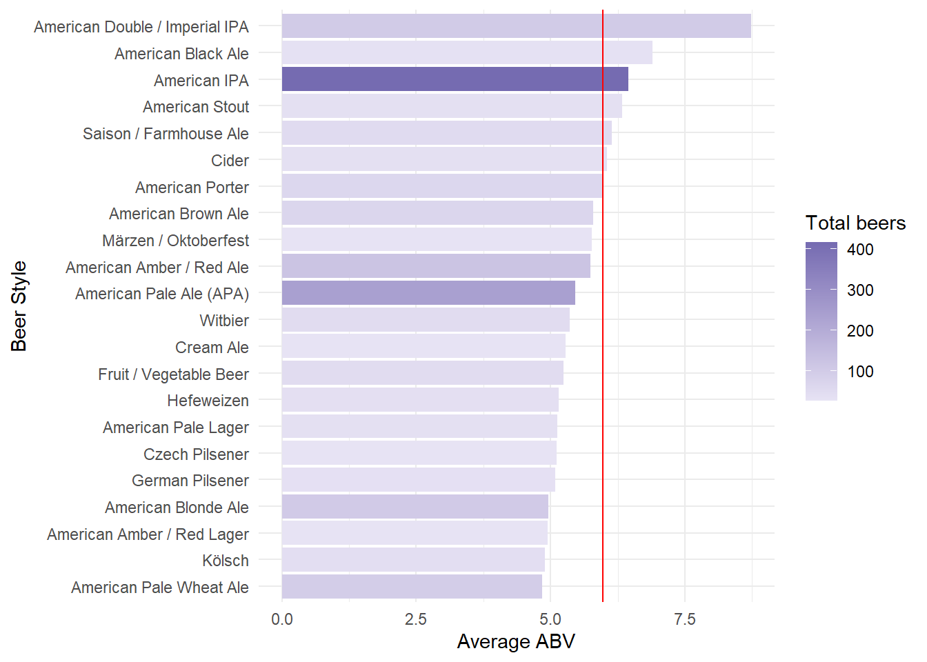
Of the popular craft beers in 2017, let’s see which styles of beer had the highest ABV.

avg_abv <- mean(beers_breweries$abv, na.rm = T)
beers_breweries %>%
  select(style, abv) %>%
  filter(complete.cases(.)) %>%
  group_by(style) %>%
  summarise(count = n(), mean_abv = mean(abv)) %>%
  filter(count > 25) %>%
  ggplot(aes(reorder(style, mean_abv), mean_abv)) + 
    geom_col(aes(fill = count)) +
    geom_hline(yintercept = avg_abv, color = 'red') + 
    coord_flip() + 
    labs(x = 'Beer Style',
         y = 'Average ABV') +
    theme_minimal() + 
    scale_fill_continuous(low = '#e7e3f4',
                          high= '#756bb1',
                          name = 'Total beers')

Linear Regression

Linear regression is one of the simplest algorithms for statistical learning. Although it may seem uninteresting compared to some of the more modern statistical learning approaches, linear regression is a useful and widely applied statistical learning method. It serves as a good starting point for more advanced approaches.

Simple Model

Let’s first create a model using the numeric variables abv, ibu, and ounces. Let’s see if we can predict abv using ibu and ounces as predictor variables.

# Get data
myvars <- c('abv', 'ibu', 'ounces')
beers_dat <- beers_breweries %>%
  select(all_of(myvars)) %>%
  filter(complete.cases(.))

# Train model
set.seed(52134)
model_simple <- train(
  abv ~ ibu + ounces, 
  data = beers_dat, 
  method = 'lm',
  trControl = trainControl(method = 'cv', number = 10)
)
print(model_simple)

## Linear Regression 
## 
## 1405 samples
##    2 predictor
## 
## No pre-processing
## Resampling: Cross-Validated (10 fold) 
## Summary of sample sizes: 1264, 1265, 1264, 1264, 1264, 1266, ... 
## Resampling results:
## 
##   RMSE      Rsquared   MAE      
##   1.001665  0.4548725  0.7174547
## 
## Tuning parameter 'intercept' was held constant at a value of TRUE

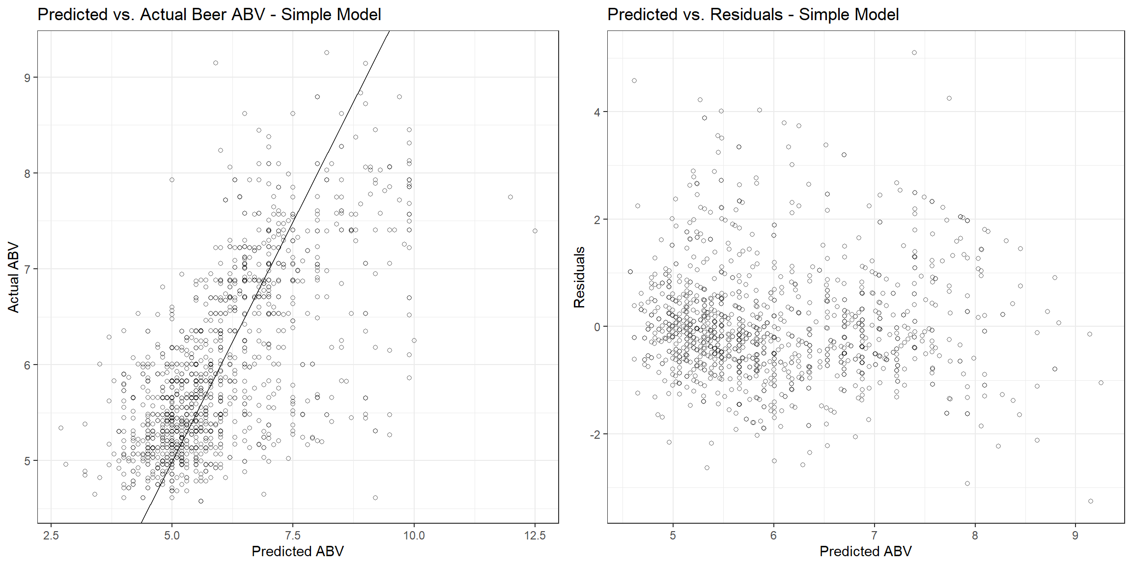
The root mean square error (RMSE), r-squared, and mean absolute error (MAE) are 1.00, 0.455, and 0.717, respectively. Let’s see how the fitted values compare to the actual values and the residuals associated with each observation.

p1 <- beers_dat %>%
  add_column(predictions = predict(model_simple, beers_dat)) %>%
  ggplot(aes(abv, predictions)) + 
  geom_point(shape = 1, size = 1.5, alpha = 0.6) +
  geom_abline() +
  labs(title = 'Predicted vs. Actual Beer ABV - Simple Model',
       x = 'Predicted ABV',
       y = 'Actual ABV') +
  theme_bw()

df1 <- broom::augment(model_simple$finalModel, data = beers_dat)
p2 <- ggplot(df1, aes(.fitted, .std.resid)) + 
  geom_point(shape = 1, size = 1.5, alpha = 0.6) +
  labs(title = 'Predicted vs. Residuals - Simple Model',
       x = 'Predicted ABV',
       y = 'Residuals') +
  theme_bw()

gridExtra::grid.arrange(p1, p2, nrow = 1)

caret Model

Now, let’s use the caret R package for regression using both numerical and categorical variables. The caret package (short for Classification And REgression Training) is a set of functions that attempt to streamline the process for creating predictive models. The package contains tools for:

• data splitting
• pre-processing
• feature selection
• model tuning using resampling
• variable importance estimation

The function dummyVars in the caret package can be used to generate a complete (less than full rank parameterized) set of dummy variables from one or more factors. The function takes a formula and a data set and outputs an object that can be used to create the dummy variables using the predict method. This parameterization is called less than full rank encoding because each factor has a dummy variable for each level. This creates perfect collinearity which may cause problems with some statistical learning algorithms (e.g., ordinary linear regression and neural networks). A full-rank encoding can be obtained by dropping one of the levels. We can use fullrank = T to create only n-1 columns for a categorical column with n different levels.

Some of our variables contain levels that have very few observations. It often is beneficial to callapse, or “lump” these levels into a lesser number of levels. However, lumping should be used sparingly as there is often a loss in model performance. For this example, we will use a single categorical variable, beer style, and not concern ourselves with low frequency of observations.

# Get data
myvars <- c('abv', 'ibu', 'ounces', 'style')
beers_dat <- beers_breweries %>%
  select(all_of(myvars)) %>%
  filter(complete.cases(.))

# Creating dummy variables
dummies_model <- dummyVars(abv ~ ., data = beers_dat, fullRank = T)

# Create the dummy variables using predict.
beers_dat_mat <- predict(dummies_model, newdata = beers_dat)

# Convert to dataframe
abv <- beers_dat %>%
  select(abv) %>%
  unlist(use.names = FALSE)
beers_dat <- data.frame(beers_dat_mat) %>%
  add_column(abv = abv) %>%
  select(abv, everything())

Now that we have a full-rank encoding of the style variable, let’s train the model.

set.seed(52134)
model_caret <- train(
  abv ~ ., 
  data = beers_dat, 
  method = 'lm',
  trControl = trainControl(method = 'cv', number = 10)
)
print(model_caret)

## Linear Regression 
## 
## 1403 samples
##   91 predictor
## 
## No pre-processing
## Resampling: Cross-Validated (10 fold) 
## Summary of sample sizes: 1262, 1263, 1262, 1262, 1262, 1264, ... 
## Resampling results:
## 
##   RMSE       Rsquared   MAE     
##   0.7733022  0.6741768  0.563042
## 
## Tuning parameter 'intercept' was held constant at a value of TRUE

The RMSE, r-squared, and MAE are 0.773, 0.674, and 0.563, respectively. Let’s see how the fitted values compare to the actual values and the residuals associated with each observation.

p1 <- beers_dat %>%
  add_column(predictions = predict(model_caret, beers_dat)) %>%
  ggplot(aes(abv, predictions)) + 
  geom_point(shape = 1, size = 1.5, alpha = 0.6) +
  geom_abline() +
  labs(title = 'Predicted vs. Actual Beer ABV - Caret Model',
       x = 'Predicted ABV',
       y = 'Actual ABV') +
  theme_bw()

df1 <- broom::augment(model_caret$finalModel, data = beers_dat)
p2 <- ggplot(df1, aes(.fitted, .std.resid)) + 
  geom_point(shape = 1, size = 1.5, alpha = 0.6) +
  labs(title = 'Predicted vs. Residuals - Caret Model',
       x = 'Predicted ABV',
       y = 'Residuals') +
  theme_bw()

gridExtra::grid.arrange(p1, p2, nrow = 1)

vtreat Model

Now, let’s perform the same regression but use the vtreat R package for encoding the categorical variable. The vtreat package is a processor/conditioner that prepares messy real-world data for statistical learning. It is designed to deal with most of the common issues encountered when modeling messy data. The vtreat process creates a treatment plan that records all the information needed to repeat the data treatment process. This treatment plan can then be used to “prepare” or treat training data before fitting a model, and then again to treat new data before feeding it into the model.

Let’s use vtreat to design a treatment plan for our beers and breweries data.

# Get data
myvars <- c('abv', 'ibu', 'ounces', 'style')
beers_dat <- beers_breweries %>%
  select(all_of(myvars)) %>%
  filter(complete.cases(.))

# Design treatment plan
treatment_plan <- designTreatmentsN(
  beers_dat, 
  colnames(beers_dat),
  outcomename = 'abv',
  codeRestriction = c('lev', 'catN', 'clean', 'isBAD')
)

## [1] "vtreat 1.6.3 inspecting inputs Wed Mar 16 20:38:13 2022"
## [1] "designing treatments Wed Mar 16 20:38:13 2022"
## [1] " have initial level statistics Wed Mar 16 20:38:13 2022"
## [1] " scoring treatments Wed Mar 16 20:38:13 2022"
## [1] "have treatment plan Wed Mar 16 20:38:13 2022"
## [1] "rescoring complex variables Wed Mar 16 20:38:13 2022"
## [1] "done rescoring complex variables Wed Mar 16 20:38:13 2022"

Now that we have designed the treatment plan, let’s use it to prepare (transform) the data into all numerical and one-hot-encoded variables.

beers_dat_trt <- prepare(treatment_plan, beers_dat)

Using the prepared data, let’s train the model.

set.seed(52134)
model_vtreat <- train(
  abv ~ ., 
  data = beers_dat_trt, 
  method = "lm", 
  trControl = trainControl(method = "cv", number = 10)
)

print(model_vtreat)

## Linear Regression 
## 
## 1403 samples
##   12 predictor
## 
## No pre-processing
## Resampling: Cross-Validated (10 fold) 
## Summary of sample sizes: 1262, 1263, 1262, 1262, 1262, 1264, ... 
## Resampling results:
## 
##   RMSE       Rsquared   MAE      
##   0.7255873  0.7127488  0.5354519
## 
## Tuning parameter 'intercept' was held constant at a value of TRUE

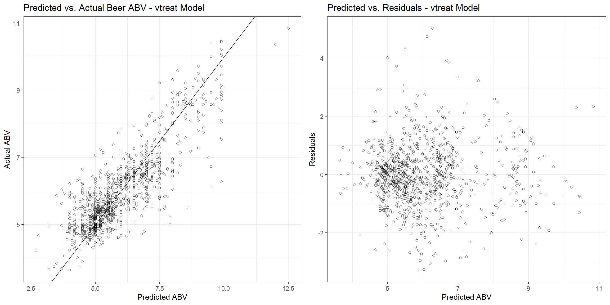
The RMSE, r-squared, and MAE are 0.726, 0.713, and 0.535, respectively. Let’s see how the fitted values compare to the actual values and the residuals associated with each observation.

p1 <- beers_dat_trt %>%
  add_column(predictions = predict(model_vtreat, beers_dat_trt)) %>%
  ggplot(aes(abv, predictions)) + 
  geom_point(shape = 1, size = 1.5, alpha = 0.6) +
  geom_abline() +
  labs(title = 'Predicted vs. Actual Beer ABV - vtreat Model',
       x = 'Predicted ABV',
       y = 'Actual ABV') +
  theme_bw()

df1 <- broom::augment(model_vtreat$finalModel, data = beers_dat_trt)
p2 <- ggplot(df1, aes(.fitted, .std.resid)) + 
  geom_point(shape = 1, size = 1.5, alpha = 0.6) +
  labs(title = 'Predicted vs. Residuals - vtreat Model',
       x = 'Predicted ABV',
       y = 'Residuals') +
  theme_bw()

gridExtra::grid.arrange(p1, p2, nrow = 1)

recipes Model

Now, let’s perform the same regression but using the recipes R package for encoding the categorical variable. The recipes package is an alternative method for creating and preprocessing design matrices that can be used for statistical learning or visualization. A design matrix (also known as regressor matrix or model matrix) is a matrix of values of explanatory variables of a set of objects. Each row represents an individual object, with the successive columns corresponding to the variables and their specific values for that object. The idea of the recipes package is to define a recipe or blueprint that can be used to sequentially define the encodings and preprocessing of the data (i.e., feature engineering).

There are three main steps in using the recipes package:

• recipe: define feature engineering steps to create the blueprint
• prepare: estimate feature engineering parameters based on training data
• bake: apply the blueprint to new data

Let’s apply these concepts to the beers and breweries data. First, we will define the blueprint (create the recipe) for use on our data. Note that one-hot or dummy encoding is performed with the same step_dummy function in the recipes package. By default, step_dummy will create a full-rank encoding but this can be changed by setting one_hot = TRUE.

# Get data
myvars <- c('abv', 'ibu', 'ounces', 'style')
beers_dat <- beers_breweries %>%
  select(all_of(myvars)) %>%
  filter(complete.cases(.))

# Create a blueprint
library(recipes)
blueprint <- recipe(abv ~ ., data = beers_dat) %>%
  step_dummy(all_nominal(), one_hot = FALSE)
blueprint

## Recipe
## 
## Inputs:
## 
##       role #variables
##    outcome          1
##  predictor          3
## 
## Operations:
## 
## Dummy variables from all_nominal()

Next, we will train (prepare) the blueprint using our data.

prepare <- prep(blueprint, training = beers_dat)
prepare

## Recipe
## 
## Inputs:
## 
##       role #variables
##    outcome          1
##  predictor          3
## 
## Training data contained 1403 data points and no missing data.
## 
## Operations:
## 
## Dummy variables from style [trained]

Finally, we apply (bake) the blueprint on our modeling data.

beers_dat_baked <- bake(prepare, new_data = beers_dat)

Using the preapred (baked) data, let’s train the model.

model_recipes <- train(
  abv ~ ., 
  data = beers_dat_baked, 
  method = "lm", 
  trControl = trainControl(method = "cv", number = 10)
)
print(model_recipes)

## Linear Regression 
## 
## 1403 samples
##   91 predictor
## 
## No pre-processing
## Resampling: Cross-Validated (10 fold) 
## Summary of sample sizes: 1262, 1263, 1263, 1263, 1263, 1262, ... 
## Resampling results:
## 
##   RMSE       Rsquared  MAE      
##   0.7810419  0.668083  0.5653162
## 
## Tuning parameter 'intercept' was held constant at a value of TRUE

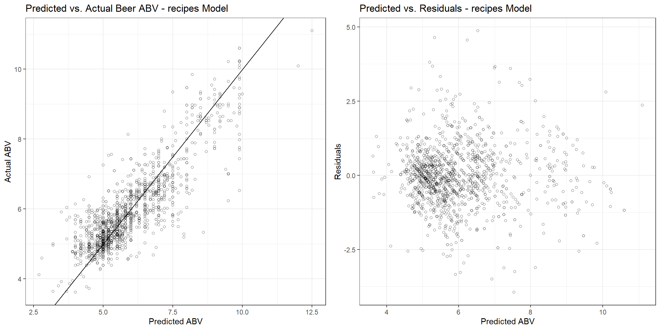
The RMSE, r-squared, and MAE are 0.781, 0.668, and 0.565, respectively. Let’s see how the fitted values compare to the actual values and the residuals associated with each observation.

p1 <- beers_dat_baked %>%
  add_column(predictions = predict(model_recipes, beers_dat_baked)) %>%
  ggplot(aes(abv, predictions)) + 
  geom_point(shape = 1, size = 1.5, alpha = 0.6) +
  geom_abline() +
  labs(title = 'Predicted vs. Actual Beer ABV - recipes Model',
       x = 'Predicted ABV',
       y = 'Actual ABV') +
  theme_bw()

df1 <- broom::augment(model_recipes$finalModel, data = beers_dat_baked)
p2 <- ggplot(df1, aes(.fitted, .std.resid)) + 
  geom_point(shape = 1, size = 1.5, alpha = 0.6) +
  labs(title = 'Predicted vs. Residuals - recipes Model',
       x = 'Predicted ABV',
       y = 'Residuals') +
  theme_bw()

gridExtra::grid.arrange(p1, p2, nrow = 1)

Conclusions

Data preprocessing and engineering techniques generally refer to the addition, deletion, or transformation of data. The time spent on identifying data engineering needs can be significant and requires the data scientist to spend substantial time understanding their data. Different models have different sensitivities to the type of target and feature values in the model. Most models require that the predictors take numeric form. This factsheet has explored several methods that can be used to encode categorical variables.

It is essential to understand these encoding methods do not work well in all situations or for every dataset. Data ccientists still need to experiment to identify which method works best for their specific case. If data have different classes, then some of these methods will not work as features will not be similar. There are a few benchmark publications by research communities, but the results are not conclusive, which method works best. For instance, decision tree models and their ensemble counterparts, random forests, are able to operate on both continuous and categorical variables directly. In contrast, generalized linear models and neural networks must instead transform categorical variables into some numerical analog, usually by one-hot encoding to create a new dummy variable for each level of the original variable. For linear regression, one-hot encoding with n-1 binary variables should be used to ensure the correct number of degrees of freedom.

One-hot encoding can lead to a huge increase in the dimensionality of the feature representations. For example, one-hot encoding U.S. states adds 49 dimensions to the intuitive feature representation. In addition, one-hot encoding can eliminate important structure in the underlying representation by splitting a single feature into many separate ones. My recommendation is to try different methods of categorical variable encoding with a small dataset prior to focusing on tuning of the statistical learning process.