Introduction

Regression is a fundamental procedure used in data analysis. Most regression analyses for quantitative data are performed by using a dependent variable for which all observations are known. However, there are certain challenges when performing regression on a dependent variable that includes censored values. A censored variable has a large fraction of observations at the minimum or maximum values. Because the censored variable is not observed over its entire range, ordinary estimates of the mean and variance will be biased. Ordinary least squares (OLS) estimates of its regression on a set of explanatory variables will also be biased and inconsistent.

The term “censored data” refers to observations that are not quantified but are known only to exceed or to be less than a threshold value. Values known only to be below a threshold are left-censored data, values known only to exceed a threshold are right-censored data, and values known only to be within an interval are interval-censored data. Environmental data are dominantly left-censored, containing multiply censored values as detection limit thresholds change over time or with varying sample characteristics. Examples of right-censored environmental data include estimates of minimum flood magnitudes and transmissivity.

Common practices for handling censored data include deletion of the censored observations or substituting nondetects with arbitrary constants, generally based on some fraction of the detection limit (DL), prior to data analysis (Krishnamoorthy et al. 2009; Lubin et al. 2004; Thompson & Nelson 2003). These approaches have been shown to distort regression coefficients (Lyles et al. 2001) and are regarded as bias-prone, lacking sound statistical justification (Gleit 1985; Newman et al. 1989; Helsel 2012; Kafatos et al 2013).

The worst practice when dealing with censored observations is to exclude or delete them. This produces a strong bias in all subsequent analysis. While better than deleting censored observations, substituting artificial values as if these had been measured provides its own inaccuracies. Ad-hoc substitution introduces structure to the data that is not in the actual population. Substitutions impose new patterns of variation on the data, making estimates inconsistent and yielding potentially misleading results. Helsel (2012) provides an example of a straight-line relationship between two variables, where the slope of the relationship is significant, with a strong positive correlation between the variables. When using one-half the DL for nondetects, the slope is dramatically changed, decreasing the correlation coefficient between the variables from 0.81 to 0.55.

Maximum Likelihood Regression

When data contain censored values, it is often necessary to use a censored regression approach rather than conventional OLS regression (Lawless 1982; Green 1990). There are several methods for incorporating censored observations into linear models. Maximum likelihood estimates (MLE) is one method of computing a regression with censored data without resorting to simple substitution. MLE methods provide a best-fit line for data with one or more reporting limits, assuming the residuals follow the chosen distribution. Censored regression using MLE is sometimes referred to as “Tobit analysis” after the economist Tobin (1958).

MLE can be used when data are left-censored, right-censored, or both left- and right-censored. The model is estimated by maximum likelihood (ML) assuming a distribution of the error term. When the censored regression model is estimated, the log-likelihood function is maximized with respect to the coefficients and the logarithm(s) of the variance(s), producing the coefficients with the highest likelihood of matching the observed data, both censored and uncensored (Helsel 2012). ML methods are used to compute regression models in a variety of disciplines, including reliability analysis, economics, medical studies, and hazard analysis.

Comparison of Censored and OLS Regression

Let’s consider an example of using both MLE and OLS for regression on censored data. We will use data that have been censored both at the minimum values (left-censored) and at the maximum values (right-censored). The results would be similar if we considered left-censored data without censoring at the maximum values.

For the analyses, let’s create a computer-generated data set containing two variables having the following regression properties:

• slope equal to 0.005
• intercept equal to -0.001
• standard error equal to 0.005

# Load libraries
library(magrittr)
library(censReg)

# Create data
set.seed(157)
n.data <- 1000
coeff <- c(-0.001, 0.005)
sigma <- 0.005
x <- rnorm(n.data, 0.5)
y <- as.vector(coeff %*% rbind(rep(1, n.data), x) + rnorm(n.data, 0, sigma))
y.cen <- y
y.cen[y < 0] <- 0
y.cen[y > 0.01] <- 0.01
dat <- data.frame(list(x = x, y = y, y.cen = y.cen))

Let’s inspect the data.

library(summarytools)

print(
  dfSummary(
    dat,
    varnumbers   = FALSE,
    valid.col    = FALSE,
    na.col = FALSE,
    style        = 'grid',
    plain.ascii  = FALSE,
    headings     = FALSE,
    graph.magnif = 0.8
  ),
  footnote = NA,
  method = 'render'
)

Let’s plot both y and y_cen as function of x.

# Let's plot the data
par(mfrow = c(1, 2))
plot(y ~ x, pch = 19, cex = 0.7, col = 'grey60', main = 'Hypothetical Data')
plot(y.cen ~ x, pch = 19, cex = 0.7, col = 'grey60', main = 'Censored Data')

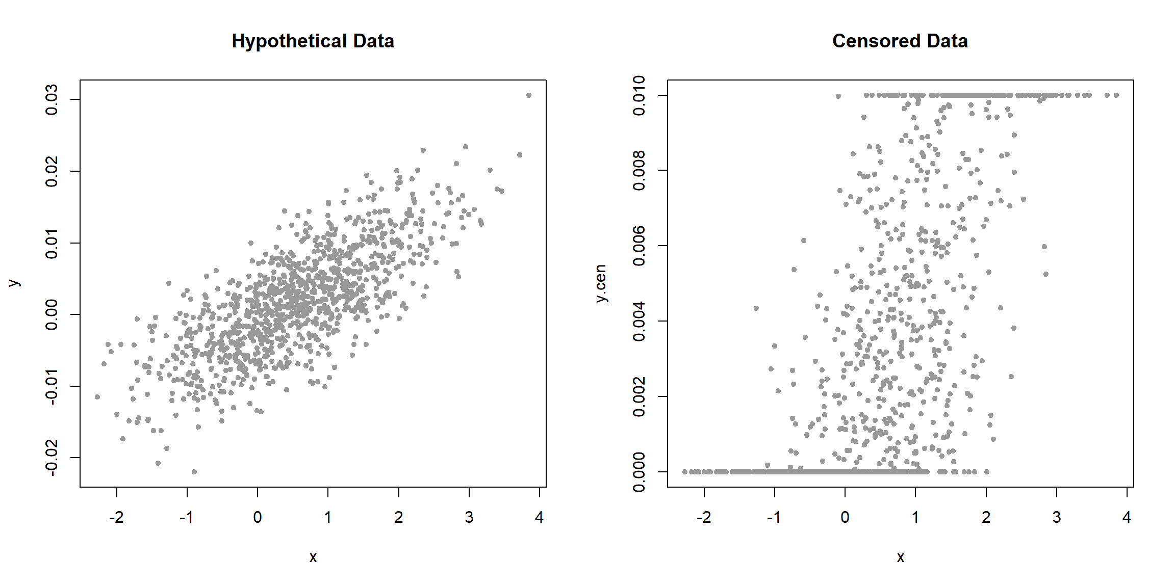
When the data are plotted using the two censoring limits of 0 and 0.01, the result includes two horizontal lines of substituted values. The pattern being added to the data is quite different than the pattern of the data itself, obscuring the original pattern of the raw, uncensored data.

Let’s fit a line to the censored data using censored regression.

# Fit a line using censored regression
fit.cen <- censReg(y.cen ~ x, data = dat, left = 0.0, right = 0.01)
summary(fit.cen)

## 
## Call:
## censReg(formula = y.cen ~ x, left = 0, right = 0.01, data = dat)
## 
## Observations:
##          Total  Left-censored     Uncensored Right-censored 
##           1000            398            470            132 
## 
## Coefficients:
##               Estimate Std. error  t value  Pr(> t)    
## (Intercept) -0.0011648  0.0002524   -4.616 3.91e-06 ***
## x            0.0053100  0.0002265   23.440  < 2e-16 ***
## logSigma    -5.3652254  0.0360980 -148.629  < 2e-16 ***
## ---
## Signif. codes:  0 '***' 0.001 '**' 0.01 '*' 0.05 '.' 0.1 ' ' 1
## 
## Newton-Raphson maximisation, 17 iterations
## Return code 8: successive function values within relative tolerance limit (reltol)
## Log-likelihood: 1538.85 on 3 Df

# Get the standard error
coef(fit.cen, logSigma = FALSE)

##  (Intercept)            x        sigma 
## -0.001164848  0.005309989  0.004676406

Let’s fit a line to the censored data using OLS.

# Fit a line using OLS regression
fit.OLS <- lm(y.cen ~ x, data = dat)
summary(fit.OLS)

## 
## Call:
## lm(formula = y.cen ~ x, data = dat)
## 
## Residuals:
##        Min         1Q     Median         3Q        Max 
## -0.0069342 -0.0020798 -0.0002012  0.0018972  0.0082408 
## 
## Coefficients:
##              Estimate Std. Error t value Pr(>|t|)    
## (Intercept) 1.958e-03  9.937e-05   19.70   <2e-16 ***
## x           2.476e-03  8.545e-05   28.98   <2e-16 ***
## ---
## Signif. codes:  0 '***' 0.001 '**' 0.01 '*' 0.05 '.' 0.1 ' ' 1
## 
## Residual standard error: 0.002783 on 998 degrees of freedom
## Multiple R-squared:  0.457,	Adjusted R-squared:  0.4565 
## F-statistic: 839.9 on 1 and 998 DF,  p-value: < 2.2e-16

Let’s fit a line to the detected values using OLS.

# For comparison, limit the regression to the quantified data
fit.detect <- lm(y[0 <= y & y <= 0.01] ~ x[0 <= y & y <= 0.01])
summary(fit.detect)

## 
## Call:
## lm(formula = y[0 <= y & y <= 0.01] ~ x[0 <= y & y <= 0.01])
## 
## Residuals:
##       Min        1Q    Median        3Q       Max 
## -0.005197 -0.002021 -0.000188  0.001710  0.007081 
## 
## Coefficients:
##                        Estimate Std. Error t value Pr(>|t|)    
## (Intercept)           0.0030192  0.0001783  16.929   <2e-16 ***
## x[0 <= y & y <= 0.01] 0.0014458  0.0001631   8.867   <2e-16 ***
## ---
## Signif. codes:  0 '***' 0.001 '**' 0.01 '*' 0.05 '.' 0.1 ' ' 1
## 
## Residual standard error: 0.002563 on 468 degrees of freedom
## Multiple R-squared:  0.1438,	Adjusted R-squared:  0.142 
## F-statistic: 78.63 on 1 and 468 DF,  p-value: < 2.2e-16

Now, let’s compare the results.

# Let's compare the values
rbind(
  Censored = c(coef(fit.cen)[1], coef(fit.cen)[2]),
  OLS_Full = coef(fit.OLS),
  OLS_Detects = coef(fit.detect)
) %>% round(4)

##             (Intercept)      x
## Censored        -0.0012 0.0053
## OLS_Full         0.0020 0.0025
## OLS_Detects      0.0030 0.0014

The results of the censored regression are remarkably close to the correct values of -0.001 for the intercept and 0.005 for the slope. The standard error is 0.00468, which is very close to the true value of 0.005. The results for the OLS regression are not close to the actual values. The coefficients from the censored regression are larger than those from OLS, indicating the downward bias of the coefficients resulting from OLS regression on a censored variable. The estimated standard errors reported by the OLS regressions were 0.00278 and 0.00256, less than half the true value. These kinds of biases are typical of regressions conducted on censored data.

Let’s plot the results to visually inspect the regression fits to the data.

# Plot the results
lineplot <- function() {

  # Add lines
  abline(coef(fit.cen)[1:2], col = 'Red', lwd = 2)
  abline(coef(fit.OLS), col = 'Blue', lty = 2, lwd = 2)
  abline(coef(fit.detect), col = rgb(0.2, 0.6, 0.2), lty = 3, lwd = 2)

  # Add legend
  legend(
    "topleft",
    legend = c(
      "Censored",
      "OLS",
      "OLS Detects"
    ),
    lwd = 3 * par("cex"),
    col = c("red", "blue", "green"),
    lty = c(1, 2, 3),
    text.font = 1, bty = "n",
    pt.cex = 1, cex = 0.8, y.intersp = 1.3
  )
}

par(mfrow = c(2, 2))

plot(x, y, pch = 19, cex = 0.7, col = 'grey60', main = 'Hypothetical Data')
lineplot()

plot(x, y.cen, pch = 19, cex = 0.7, col = 'grey60', main = 'Censored Data')
lineplot()

hist(y[0 <= y & y <= 0.01], breaks = 50, main = 'Quantified Data')
hist(y.cen, breaks = 50, main = 'Censored Data')

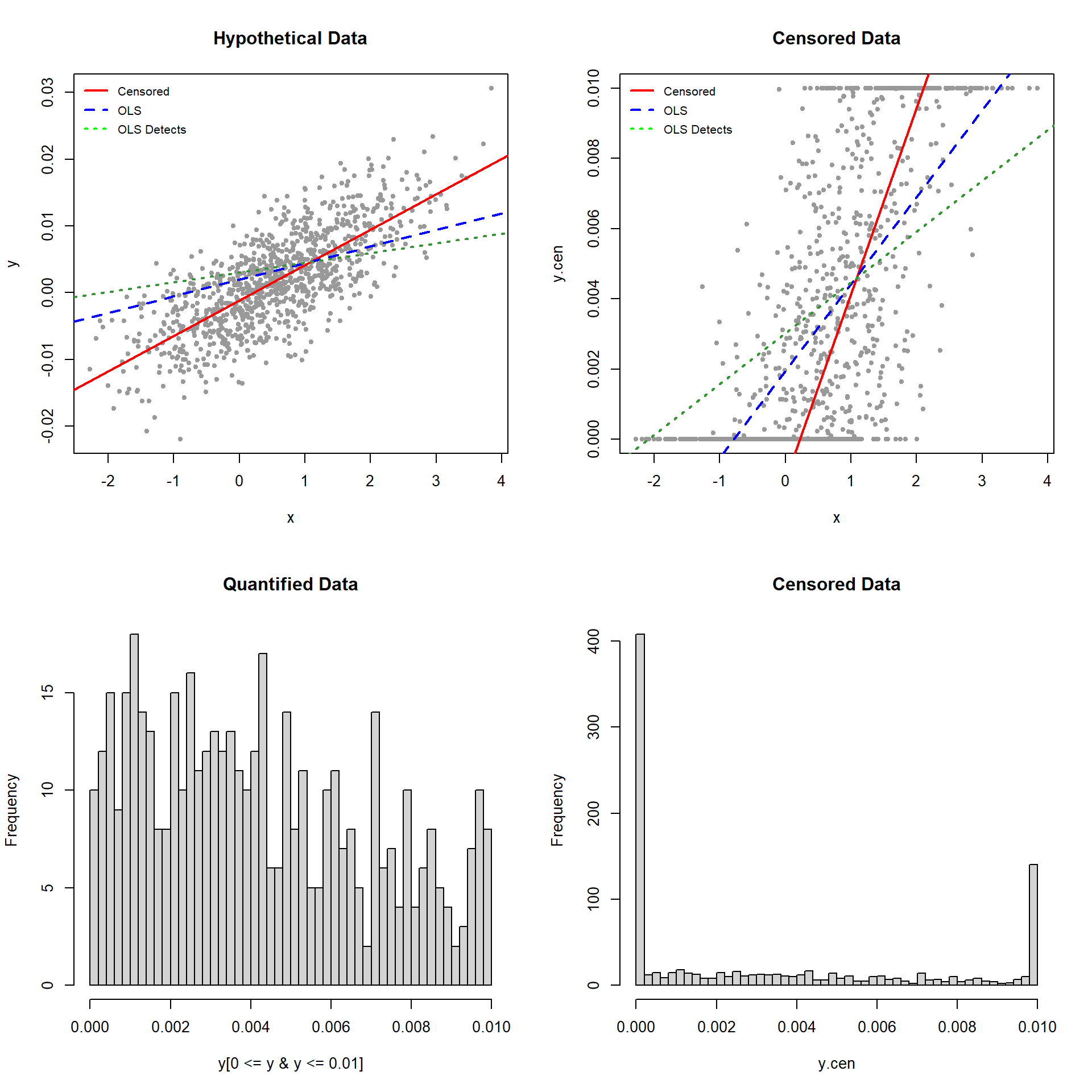
The difference between the “hypothetical data” and “censored data” plots is that all y-values below 0 or above 0.01 in the former plot have been censored to produce the latter plot. The solid red lines are the censored fits, the dashed blue lines the OLS fits substituting the censoring values for the nondetects, and the dashed green lines are the OLS fits using only the detected data (censored values ignored). The blue and green lines provide a noticeably poor fit to the data and only the red line (for the censored regression fit) fits the data.

Conclusions

Although it is easy and convenient to either ignore censored values or substitute some fraction of the DL, these approaches tend to be biased and cause a loss of information. Results for standard errors are biased, which may further distort inferences based on the regression. Censored regression methods produce more accurate and robust estimates than these bias-prone methods. MLE is one method of computing a regression with censored data without resorting to simple substitution. MLE methods provide a best-fit line for data with one or more DLs, assuming the residuals follow the chosen distribution. For skewed environmental data where most variables have values spanning two or more orders of magnitude, a lognormal distribution is most often assumed. The lognormal distribution has the additional benefit that estimated values cannot go negative, a problem that is often encountered when assuming a normal distribution for low-level contaminants.

References

Gleit, A. 1985. Estimation for small normal data sets with detection limits. Environ. Sci. Technol. 19, 1201-1206.

Greene, W.H. 1990. Econometric Analysis. Macmillan Publishing Company, New York.

Helsel, D.R. 2012. Statistics for Censored Environmental Data using Minitab and R, 2nd Edition. New York: John Wiley & Sons.

Kafatos, G., N. Andrews, K.J. McConway, and P. Farrington. 2013. Regression models for censored serological data. J Med Microbiol. 62, 93-100.

Krishnamoorthy, K., A. Mallick, and T. Mathew. 2009. Model-based imputation approach for data analysis in the presence of non-detects. Ann Occup Hyg 53, 249-263.

Lawless, J.F. 1982. Statistical Models and Methods for Lifetime Data. John Wiley & Sons, Inc. New York.

Lubin, J.H., J.S. Colt, D. Camann, S. Davis, J.R. Cerhan, JR.K. Severson, L. Bernstein, and P. Hartge. 2004. Epidemiologic evaluation of measurement data in the presence of detection limits. Environ Health Perspect 112, 1691-1696.

Lyles, R.H., D. Fan, and R. Chuachoowong. 2001. Correlation coefficient estimation involving a left censored laboratory assay variable. Stat Med 20, 2921-2933.

Newman, M.C., P.M. Dixon, B.B. Looney, J.E. Finder. 1989. Estimating mean and variance for environmental samples with below detection limit observations. Water Resour. Bull. 1989, 25, 905-915.

Thompson, M.L. and K.P. Nelson. 2003. Linear regression with Type I interval- and left-censored response data. Environ Ecol Stat 10, 221-230.

Tobin, J. 1958. Estimation of relationships for limited dependent variables. Econometrica 31, 24-36.