Introduction

This is a perfunctory exploration of the early transmission dynamics of coronavirus disease 2019 (COVID-19) in mainland China using the R statistical programming language. Since the first suspected case of COVID-19 on December 1, 2019, in Wuhan, Hubei Province, China, a total of 80,860 confirmed cases and 3,213 deaths have been reported in China up through March 15, 2020. The main epidemiological parameters including the basic reproduction number \((R_0)\) and the per day infection mortality and recovery rates are estimated using a classic SIR (Susceptible-Infectious-Recovered) compartmental model of communicable disease outbreaks.

As the number of infected individuals, especially of those with asymptomatic or mild courses, is suspected to be much higher than the official numbers, this curiosity-driven evaluation is more an example of using R for modelling communicable disease outbreaks than a complete characterization of the epidemic trajectory for COVID-19. This work has not be peer-reviewed nor do I claim any particular expertise in communicable, or infectious diseases.

Data

Let’s create a vector with the daily cumulative incidence for Mainland China, from January 16, 2020 when our daily incidence data starts, through January 31, 2020. This wikipedia page, which is currently being updated promptly as new data are released, is a detailed and well-referenced source. We’ll use this initial data to fit the model and then compare the predictions to the observe confirmed cases through March 14, 2020. We need a value for the initial uninfected population. The approximate population of mainland China in 2019 was 1,440,000,000 people, according to this wikipedia page.

# Load libraries
library(dplyr)
library(ggplot2)
library(gridExtra)
library(grid)
library(scales)
library(lubridate)
library(deSolve)
library(EpiEstim)
library(incidence)

Infected <- c(45, 62, 121, 198, 291, 440, 571, 830, 1287, 1975,
              2744, 4515, 5974, 7711, 9692, 11791)
Day <- 1:(length(Infected))
N <- 1440000000    # pop of china 1,440,000,000
sir_start_date <- "2020-01-16"

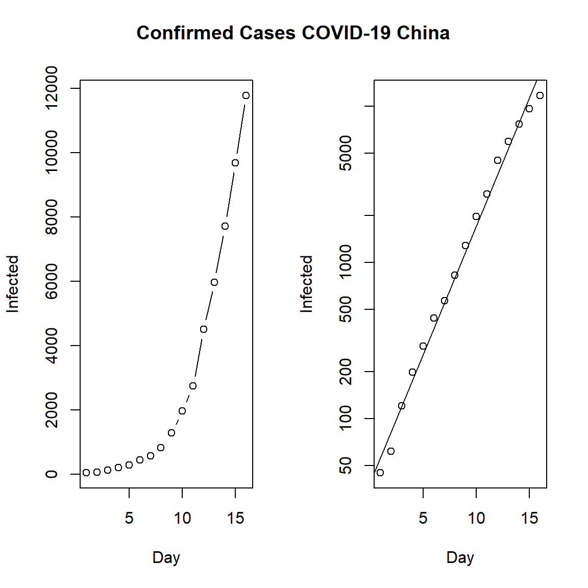
First, let’s look at the daily cumulative number of incident cases for mainland China. On the left, we see the confirmed cases in mainland China and on the right the same but using a log-linear plot. The data indicates that the epidemic was in an exponential phase during this intial period.

par(mfrow = c(1, 2))
plot(Day, Infected, type = "b")
plot(Day, Infected, log = "y")
abline(lm(log10(Infected) ~ Day))
title("Confirmed Cases COVID-19 China", outer = TRUE, line = -2)

Model

Although there are many epidemiological models available, we will use one of the simplest here, the SIR model. The SIR model is a simple epidemiology compartmental model proposed by Kermack and McKendrick (1927), which assumes a fixed population with only three compartments or states:

• S(t) = the number of individuals susceptible to the disease not yet infected at time t;

• I(t) = the number of individuals who have been infected at time t with the disease and are capable of spreading the disease to those in the susceptible category;

• R(t) = number of individuals who have been infected and then recovered from the disease, either due to immunisation or due to death.

To model the dynamics of the outbreak we need three differential equations, one for the change in each group, where \(\beta\) is the parameter that controls the transition between S and I and \(\gamma\) which controls the transition between I and R:

$$\frac{dS}{dt} = - \frac{\beta I S}{N}$$

$$\frac{dI}{dt} = \frac{\beta I S}{N}- \gamma I$$

$$\frac{dR}{dt} = \gamma I$$

The parameter N is the initial uninfected population, which we set at 1,440,000,000 people.

SIR <- function(time, state, parameters) {
    par <- as.list(c(state, parameters))
    with(par, {
        dS <- -beta * I * S/N
        dI <- beta * I * S/N - gamma * I
        dR <- gamma * I
        list(c(dS, dI, dR))
    })
}

Next, we will specify the initial values for S, I, and R.

init <- c(S = N - Infected[1], I = Infected[1], R = 0)

We need to define a function to calculate the residual sum of squares (RSS), given a set of values for \(\beta\) and \(\gamma\) to obtain the best fit to the incident data.

RSS <- function(parameters) {
    names(parameters) <- c("beta", "gamma")
    out <- ode(y = init, times = Day, func = SIR, parms = parameters)
    fit <- out[, 3]
    sum((Infected - fit)^2)
}

Finally, we can fit the SIR model to our data by finding the values for \(\beta\) and \(\gamma\) that minimise the RSS between the observed cumulative incidence and the predicted cumulative incidence. We also need to check that our model has converged.

Opt <- optim(c(0.5, 0.5), RSS, method = "L-BFGS-B",
             lower = c(0, 0), upper = c(1, 1))

# Check for convergence
Opt$message

## [1] "CONVERGENCE: REL_REDUCTION_OF_F <= FACTR*EPSMCH"

Convergence is confirmed. Now we can examine the fitted values for \(\beta\) and \(\gamma\).

Opt_par <- setNames(Opt$par, c("beta", "gamma"))
Opt_par

##      beta     gamma 
## 0.6900618 0.3099382

We can extract some interesting statistics from the model. One important number is the basic reproduction number \(R_0\), which gives the average number of susceptible people who are infected by each infectious person.

\(R_0\) is an epidemiologic metric used to describe the contagiousness or transmissibility of infectious agents. \(R_0\) is affected by numerous biological, sociobehavioral, and environmental factors that govern pathogen transmission. \(R_0\) is rarely measured directly, and modeled \(R_0\) values are dependent on model structures and assumptions. \(R_0\) must be estimated, reported, and applied with great caution because this basic metric is far from simple.

\(R_0\) has been described as being one of the fundamental and most often used metrics for the study of infectious disease dynamics. An \(R_0\) for an infectious disease event is generally reported as a single numeric value or low-high range, and the interpretation is typically presented as straightforward; an outbreak is expected to continue if \(R_0\) has a value >1 and to end if \(R_0\) is <1. The potential size of an outbreak or epidemic often is based on the magnitude of the \(R_0\) value for that event, and \(R_0\) can be used to estimate the proportion of the population that must be vaccinated to eliminate an infection from that population.

R0 <- setNames(Opt_par["beta"] / Opt_par["gamma"], "R0")
R0

##      R0 
## 2.22645

Our estimate of \(R_0\) is consistent with early estimates from other groups: 2.0 to 3.3 (Majumder and Mandl 2020); 2.6 (uncertainty range 1.5 to 3.5)(Imai et al. 2020); 2.92 (95% interval: 2.28 to 3.67) (Liu et al. 2020); 2.2 (90% interval: 1.4 to 3.8) (Riou and Althaus 2020). Because \(R_0\) values greater than 1 indicate the possibility of sustained transmission, our analysis suggests that COVID-19 exhibits epidemic potential under the assumption that currently available public information is accurate and relatively complete.

Predictions

Now, let’s make (possibly naively) predictions about the epidemic. We’ll use our model fitted to the first 16 days of available data on confirmed cases in mainland China to see what would happen if the outbreak were left to run its course, without public health interventions. We’ll compare the fitted model to actual observed incidence data through March 14, 2020.

First, let’s create a dataframe of the observed daily cumulative incidence data.

# Create dataframe with comfimed cases from 16 January through 14 March
confirmed <- c(45, 62, 121, 198, 291, 440, 571, 830, 1287, 1975,
    2744, 4515, 5974, 7711, 9692, 11791, 14380, 17205, 20440, 24324,
    28018, 31161, 34546, 37198, 40171, 42638, 44653, 59804, 63851, 66492,
    68500, 70548, 72436, 74185, 74576, 75465, 76288, 76936, 77150, 77658,
    78064, 78497, 78824, 79251, 79824, 80026, 80151, 80270, 80409, 80552,
    80651, 80695, 80735, 80754, 80778, 80793, 80813, 80824, 80844)
time <- 1:(length(confirmed))
confirmed_df <- data.frame(cbind(confirmed, time = time))

Now, we have to create a vector of time in days for predictions, and use that to get fitted values from our SIR model. After that, we will combine the model predictions with the observed daily cumulative incidence data.

# Create vector of time in days
t <- 1:70

# Get the fitted values from our SIR model
fitted_cumulative_incidence <- data.frame(ode(y = init, times = t, 
    func = SIR, parms = Opt_par))

# Add a dates column and join the observed incidence data
fitted_cumulative_incidence <- fitted_cumulative_incidence %>% 
    mutate(dates = ymd(sir_start_date) + days(t - 1)) %>%
    left_join(confirmed_df, by = "time")

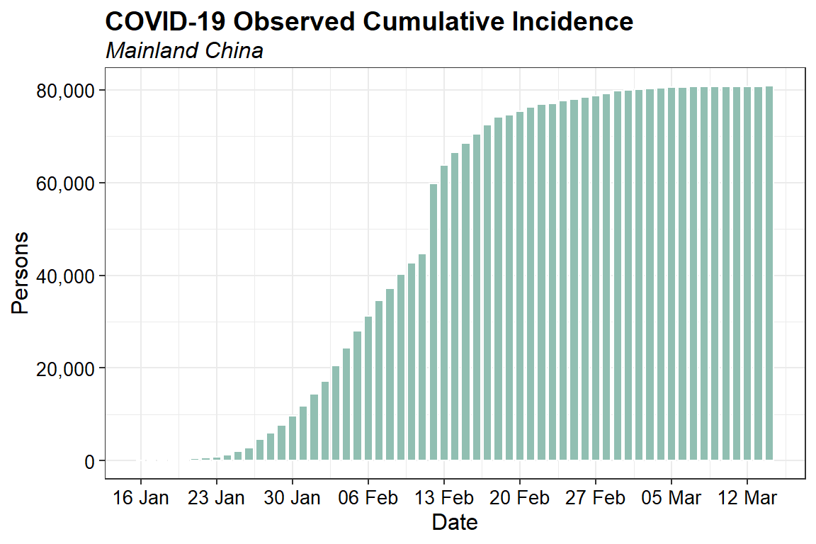
Let’s inspect the observed daily cumulative incidence data.

ggplot(data = na.omit(fitted_cumulative_incidence),
    aes(x = dates, y = confirmed)) +
    geom_bar(stat = "identity", width = 0.8, color = "white", fill = "#91BFB2") +
    scale_x_date(date_breaks="7 days", date_labels = "%d %b") +
    scale_y_continuous(labels = function(x) format(x, big.mark = ",",
                                                   scientific = FALSE)) +
    labs(title = "COVID-19 Observed Cumulative Incidence",
         subtitle = "Mainland China",
         x = "Date",
         y = "Persons") +
    theme_bw() +
    theme(plot.title = element_text(margin = margin(b = 3), size = 14,
                           hjust = 0.0, color = "black", face = quote(bold)),
          plot.subtitle = element_text(margin = margin(b = 3), size = 12,
                              hjust = 0.0, color = "black", face = quote(italic)),
          axis.title.y = element_text(size = 12, color = "black"),
          axis.title.x = element_text(size = 12, color = "black"),
          axis.text.x = element_text(size = 10, color = "black"),
          axis.text.y = element_text(size = 10, color = "black"))

Now, let’s compare the predicted incidence from the SIR model fitted to the first 16 days of data with the observed daily cumulative incidence data through March 14, 2020.

ggplot(data = fitted_cumulative_incidence, aes(x = dates)) +
    geom_line(aes(y = I, color = "red"), size = 1) +
    geom_line(aes(y = S, color = "black"), size = 1) + 
    geom_line(aes(y = R, color = "green"), size = 1) +
    geom_point(aes(y = confirmed, color = "orange"), size = 2) +
    scale_y_log10(limits = c(10, 5000000000),
                  breaks = c(100, 1000, 10000, 100000, 1000000, 10000000,
                             100000000, 1000000000),
                  expand = c(0, 0),
                  labels = function(x) format(x, big.mark = ",",
                                                   scientific = FALSE)) +
    labs(title = "COVID-19 Fitted vs Observed Cumulative Incidence",
         subtitle = "Mainland Chine",
         x = "Date",
         y = "Persons") +
    scale_color_manual(name = "",
                       values = c("red"    = "red",
                                  "black"  = "black",
                                  "green"  = "green3",
                                  "orange" = "#0A9AFA"),
                       labels = c("Susceptible", 
                                  "Recovered",
                                  "Observed",
                                  "Infectious")) +
    theme_bw() +
    theme(plot.title = element_text(margin = margin(b = 3), size = 14,
                           hjust = 0.0, color = "black", face = quote(bold)),
          plot.subtitle = element_text(margin = margin(b = 3), size = 12,
                              hjust = 0.0, color = "black", face = quote(italic)),
          axis.title.y = element_text(size = 12, color = "black"),
          axis.title.x = element_text(size = 12, color = "black"),
          axis.text.x = element_text(size = 10, color = "black"),
          axis.text.y = element_text(size = 10, color = "black")) +
    annotation_logticks(sides = "lr")

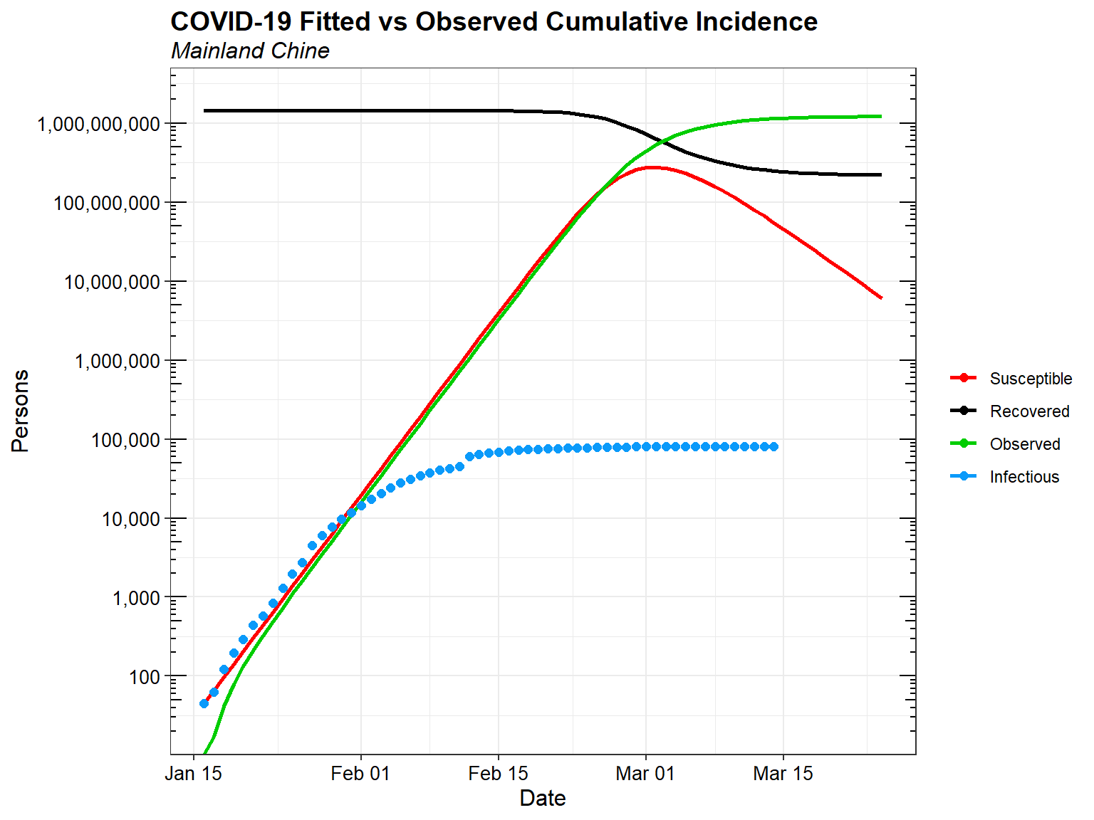
Clearly if the outbreak were left to run its course without public health interventions, it would be a disaster. Decisive public health intervention has been critical in mitigating the COVID-19 outbreak. Without such interventions, tens-of-millions of people could be infected, and even with only a one- or two-percent mortality rate, hundreds-of-thousands of people would die.

Estimating the Effective Reproduction Number

It is useful to estimate the effective reproduction number \(R_e\) on a day-by-day basis so as to track the effectiveness of public health interventions. There are several available methods for estimating \(R_e\). The EpiEstim package for R can be used to estimate the instantaneous \(R_e\).

A critical parameter for estimating the instantaneous \(R_e\) is the serial interval (SI). The SI is the time between onset of symptoms of each case of the disease in question, and the onset of symptoms in any secondary cases that result from transmission from the primary cases. The SI is a statistical distribution of serial interval times, rather than a fixed value. That distribution can be simulated, typically using a discrete gamma distribution with a given mean and standard deviation.

Li et al. estimate the SI distribution to have a mean of 7.5 days with a standard deviation (SD) of 3.4 days. These values were derived from analysis of 5 primary cases among the first 450 cases in Wuhan, China. These values are similar to the SI parameters for the Middle East respiratory syndrome coronavirus (MERS-CoV), which has a mean of 7.6 and a SD of 3.4 (Zhao et al. 2020). This similarity is not surprising given that both pathogens are coronavirii. Let’s use these values to estimate the instantaneous \(R_e\) for mainland China.

First, let’s create a dataframe with daily incidence data using the daily cumulative incidence data.

dat <- fitted_cumulative_incidence[, c("confirmed", "dates")]
dat$I <- c(dat$confirmed[1], diff(dat$confirmed))
dat <- na.omit(dat)

Let’s create a function to plot the results.

plot_Ri <- function(estimate_R_obj) {
    p_I <- plot(estimate_R_obj, "incid", add_imported_cases = TRUE)  # plots the incidence
    p_SI <- plot(estimate_R_obj, "SI")  # plots the serial interval distribution
    p_Ri <- plot(estimate_R_obj, "R")
    return(gridExtra::grid.arrange(p_I, p_SI, p_Ri, ncol = 1))
}

Let’s estimate the instantaneous \(R_e\) and plot the results.

res_parametric_si <- estimate_R(dat[, c("dates", "I")], 
    method = "parametric_si",
    config = make_config(list(mean_si = 7.5,
                              std_si = 3.4)))
plot_Ri(res_parametric_si)

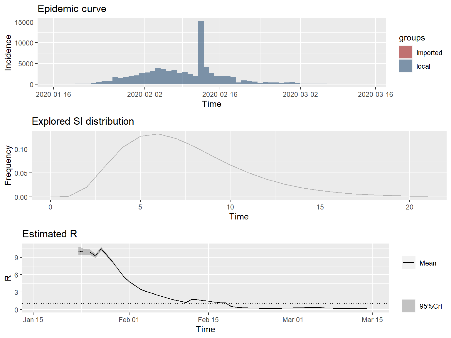
The slope of the instantaneous \(R_e\) curve is decidedly downwards, indicating that containment efforts are succeeding in progressively reducing transmission of the disease in mainland China.

Thee 7-day sliding window estimates of the instantaneous \(R_e\) are very high, approaching 10 at the peak. This seems unlikely. One possible explanation is that COVID-19 is transmissible before the onset of symptoms, resulting in much shorter SIs than expected, possibly shorter than the incubation period. Alternatively, there may be nonsymptomatic, sub-clinical spreaders of the disease, who are undetected. Another possible explanation is that there may be a great deal of variation in the SI distribution between cases.

Uncertainty in the SI distribution can be evaluated by specifying a distribution of distributions of SIs in the EpiEstim package. Let’s rerun the estimates using the mean SI estimated by Li et al. of 7.5 days, with an SD of 3.4, but allowing that mean SI to vary between 2.3 and 8.4 using a truncated normal distribution with an SD of 2.0. Let’s also allow the SD to vary between 0.5 and 4.0.

res_parametric_si <- estimate_R(dat, 
    method = "uncertain_si",
    config = make_config(list(mean_si = 7.5,
                              std_mean_si = 2.0, 
                              min_mean_si = 2.3,
                              max_mean_si = 8.4,
                              std_si = 3.4,
                              std_std_si = 1, 
                              min_std_si = 0.5,
                              max_std_si = 4,
                              n1 = 1000,
                              n2 = 1000)))
plot_Ri(res_parametric_si)

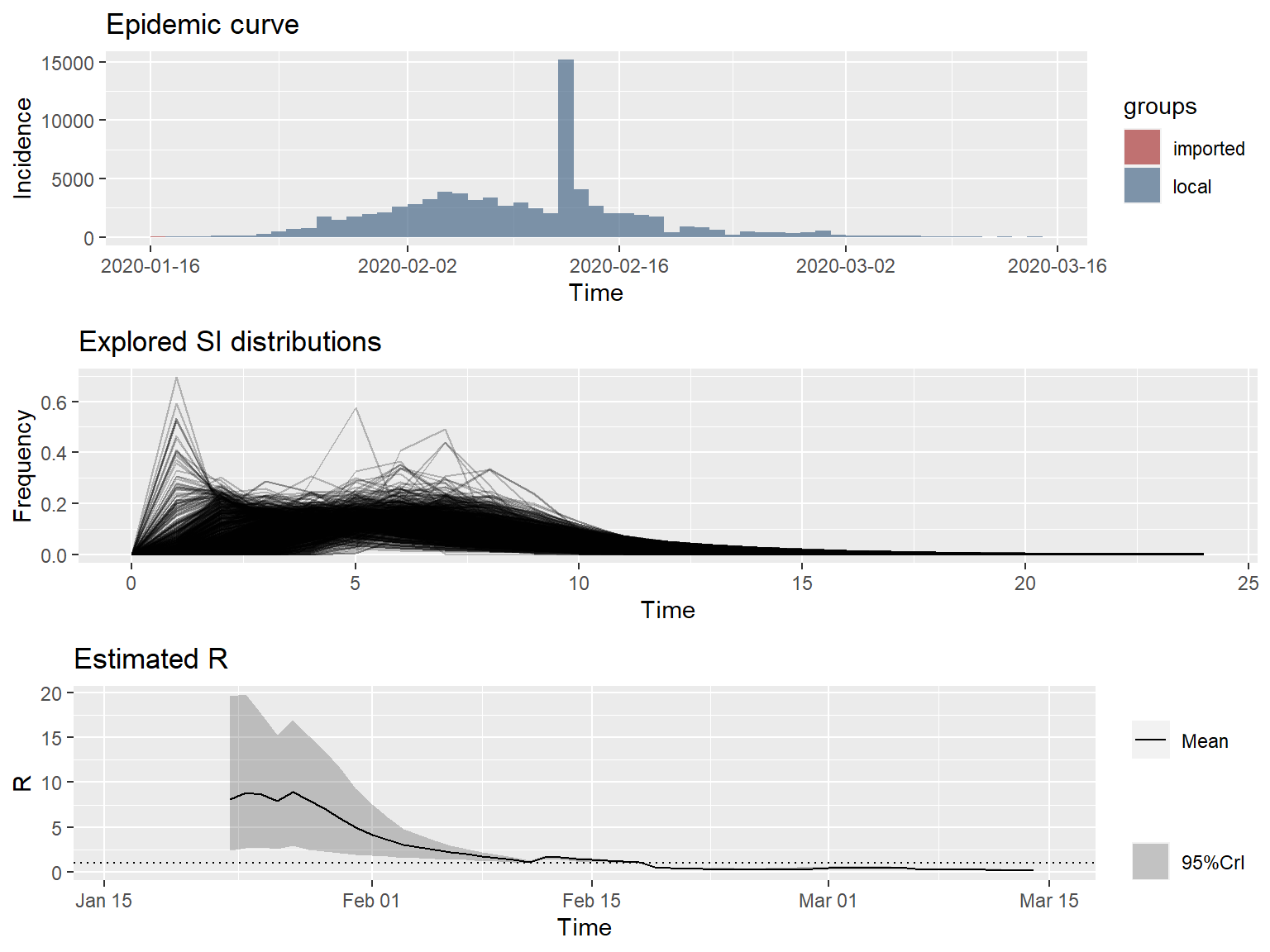
These \(R_e\) values look more reasonable, and clearly indicate that \(R_e\) is declining in mainland China, no matter what distribution is used for the SI.

Conclusions

It appears that China has mitigated the spread of the COVID-19 virus through decisive public health action and implementing strict social isolation policies. How long these measures will need to remain in place is unclear, but could be estimated using methods similar to those described above. The results of this analysis should be considered a perfunctory exploration of the early transmission dynamics of COVID-19 in mainland China. The transmission dynamics of COVID-19 are likey to change as more data became available to support more advanced modelling approaches.

References

Imai, N. et al. 2020. Transmissibility of 2019-nCoV. Imperial College.

Kermack, W. O. and A. G. McKendrick. 1927. A contribution to the mathematical theory of epidemics. Proceedings of the Royal Society A: Mathematical, Physical and Engineering Sciences 115, 700-721.

Li, Q. et al. 2020. Early Transmission Dynamics in Wuhan, China, of Novel Coronavirus-Infected Pneumonia. New England Journal of Medicine. DOI: 10.1056/NEJMoa2001316.

Liu, T. et al. 2020. Transmission Dynamics of 2019 Novel Coronavirus (2019-nCoV). bioRxiv. doi: 10.1101/2020.01.25.919787.

Majumder, M. and Mandl, K. D. 2020. Early Transmissibility Assessment of a Novel Coronavirus in Wuhan, China. Available at: https://papers.ssrn.com/abstract=3524675.

Riou, J. and Althaus, C. L. 2020. Pattern of Early Human-to-Human Transmission of Wuhan 2019-nCoV. bioRxiv 2020.01.23.917351. Available at: https://www.biorxiv.org/content/10.1101/2020.01.23.917351v1.full.pdf.

Zhao, S., Q. Lin, J. Ran, S.S. Musa, G. Yang, W. Wang, Y. Lou, D. Gao, L. Yang, D. He, and M. Wang. 2020. Preliminary estimation of the basic reproduction number of novel coronavirus (2019-nCoV) in China, from 2019 to 2020: A data-driven analysis in the early phase of the outbreak. International Journal of Infectious Diseases 92, 214-217.