Introduction

The R statistical environment and programming language is a valuable tool for conducting geospatial analysis, manipulating geographical information, and for the production of maps. An important aspect of these types of analysis is communicating the results. This example will briefly outline basic commands for producing maps using R. First, we will create several basic static maps using the functionalities provided by a few different R packages. Then, we will create a more complex map containing many different layers. There are several R packages for creating static maps, including the ggplot2, tmap, and ggmap packages for static maps. In addition to creating static maps, there also are many packages in R for creating interactive maps (leaflet, tmap, and mapview packages) and animated maps (animation, gganimate, and tmap packages). For this example, we will mainly focus on creating the map and not necessarily on the plethora of elements that are available for enhancing the visual aesthetics of the map. Although the last example does illustrate how to create a visually appealling map using R.

Data

First, let’s load a weekly earthquake dataset that can be downloaded from https://earthquake.usgs.gov/earthquakes/feed/v1.0/summary/all_week.csv. This file is updated daily and consists of the last seven days of data collection.

# Load libraries
library(ggplot2)
library(ggmap)
library(ggsn)
library(dplyr)
library(lubridate)
library(sf)
library(spData)
library(tmap)
library(mapview)
library(ggthemes)
library(av)
library(ggsn)

# Load data
quakes <- read.csv(
  "./data/all_week.csv", header = TRUE,
  stringsAsFactors = FALSE
)
str(quakes)

## 'data.frame':	3362 obs. of  22 variables:
##  $ time           : chr  "2019-09-15T18:02:10.120Z" "2019-09-15T18:00:33.550Z" "2019-09-15T17:56:04.833Z" "2019-09-15T17:52:09.910Z" ...
##  $ latitude       : num  35.7 35.6 60.2 38.8 35.7 ...
##  $ longitude      : num  -117 -117 -141 -123 -117 ...
##  $ depth          : num  4.45 4.82 3.6 2.8 1.31 ...
##  $ mag            : num  1.62 2.05 1.6 0.56 2.13 0.93 1.48 1.2 0.54 0.8 ...
##  $ magType        : chr  "ml" "ml" "ml" "md" ...
##  $ nst            : int  26 30 NA 13 36 13 17 NA 21 NA ...
##  $ gap            : num  52 84 NA 82 65 116 119 NA 59 NA ...
##  $ dmin           : num  0.0525 0.0365 NA 0.0117 0.0663 ...
##  $ rms            : num  0.18 0.15 1.01 0.04 0.15 0.21 0.24 0.74 0.11 0.76 ...
##  $ net            : chr  "ci" "ci" "ak" "nc" ...
##  $ id             : chr  "ci38838255" "ci38838247" "ak019buz3x5v" "nc73274205" ...
##  $ updated        : chr  "2019-09-15T18:06:06.296Z" "2019-09-15T18:11:09.760Z" "2019-09-15T18:01:02.191Z" "2019-09-15T18:11:02.617Z" ...
##  $ place          : chr  "14km SSW of Searles Valley, CA" "16km S of Searles Valley, CA" "62km E of Cape Yakataga, Alaska" "6km WNW of The Geysers, CA" ...
##  $ type           : chr  "earthquake" "earthquake" "earthquake" "earthquake" ...
##  $ horizontalError: num  0.27 0.22 NA 0.38 0.22 0.91 0.63 NA 0.21 NA ...
##  $ depthError     : num  0.62 0.36 0.4 0.95 0.54 0.52 1.28 0.3 0.62 0.3 ...
##  $ magError       : num  0.138 0.175 NA 0.39 0.243 0.248 0.186 NA 0.082 NA ...
##  $ magNst         : int  22 26 NA 2 27 28 30 NA 15 NA ...
##  $ status         : chr  "automatic" "automatic" "automatic" "automatic" ...
##  $ locationSource : chr  "ci" "ci" "ak" "nc" ...
##  $ magSource      : chr  "ci" "ci" "ak" "nc" ...

Let’s assign variable types to the data and then filter out any non-earthquake data.

quakes$time <- ymd_hms(quakes$time)
quakes$updated <- ymd_hms(quakes$updated)
quakes$magType <- as.factor(quakes$magType)
quakes$net <- as.factor(quakes$net)
quakes$type <- as.factor(quakes$type)
quakes$status <- as.factor(quakes$status)
quakes$locationSource <- as.factor(quakes$locationSource)
quakes$magSource <- as.factor(quakes$magSource)
quakes <- arrange(quakes, -row_number())

# earthquakes dataset
earthquakes <- quakes %>%
  filter(type == "earthquake")
str(earthquakes)

## 'data.frame':	3316 obs. of  22 variables:
##  $ time           : POSIXct, format: "2019-09-08 18:17:57" "2019-09-08 18:18:31" ...
##  $ latitude       : num  36.1 37.6 35.8 35.7 36.1 ...
##  $ longitude      : num  -118 -119 -118 -118 -118 ...
##  $ depth          : num  0.91 -1.1 4.6 7.95 1.96 ...
##  $ mag            : num  0.76 0.44 0.64 0.44 0.69 0.91 1.1 2.63 2.08 1.3 ...
##  $ magType        : Factor w/ 8 levels "mb","mb_lg","md",..: 5 3 5 5 5 5 5 5 5 5 ...
##  $ nst            : int  10 10 7 7 12 13 NA 65 31 11 ...
##  $ gap            : num  100 266 108 184 75 ...
##  $ dmin           : num  0.047 0.0385 0.0585 0.1109 0.0452 ...
##  $ rms            : num  0.15 0.07 0.16 0.13 0.11 ...
##  $ net            : Factor w/ 15 levels "ak","av","ci",..: 3 7 3 3 3 3 1 4 3 9 ...
##  $ id             : chr  "ci38819767" "nc73267625" "ci38819775" "ci38819791" ...
##  $ updated        : POSIXct, format: "2019-09-08 18:21:30" "2019-09-09 23:51:03" ...
##  $ place          : chr  "14km ENE of Coso Junction, CA" "15km W of Toms Place, CA" "24km ESE of Little Lake, CA" "13km NE of Ridgecrest, CA" ...
##  $ type           : Factor w/ 6 levels "earthquake","explosion",..: 1 1 1 1 1 1 1 1 1 1 ...
##  $ horizontalError: num  0.4 1.23 0.45 1.14 0.64 0.3 NA 0.39 0.21 NA ...
##  $ depthError     : num  0.55 0.55 1.17 1.74 0.94 0.8 0.4 0.47 0.46 0 ...
##  $ magError       : num  0.242 0.342 0.178 0.156 0.269 0.169 NA 0.161 0.142 0.1 ...
##  $ magNst         : int  5 10 8 6 3 8 NA 33 26 7 ...
##  $ status         : Factor w/ 2 levels "automatic","reviewed": 1 2 1 1 1 1 1 2 1 2 ...
##  $ locationSource : Factor w/ 15 levels "ak","av","ci",..: 3 7 3 3 3 3 1 4 3 9 ...
##  $ magSource      : Factor w/ 16 levels "ak","av","ci",..: 3 8 3 3 3 3 1 5 3 10 ...

Basic Static Maps

Static maps are the most common type of visual output from geocomputation. For this example,we will create static maps using the functionalities provided within the ggplot2, tmap, and ggmap packages.

ggplot2 Package

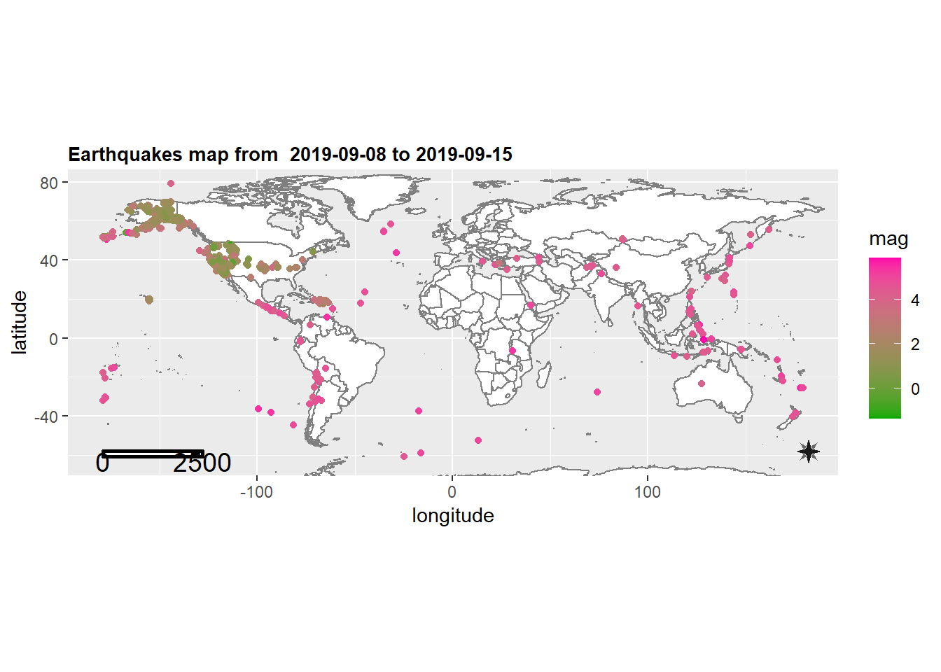
Let’s create a static map of the earthquake events using the ggplot package.

world <- map_data('world')
title <- paste(
  "Earthquakes map from ",
  paste(
    as.Date(earthquakes$time[1]),
    as.Date(earthquakes$time[nrow(earthquakes)]
  ),
  sep = " to ")
)

p <- ggplot() + 
  geom_map(data = world, map = world,
           aes(group = group, map_id = region),
           fill = "white", color = "#7f7f7f", size = 0.5) +
  geom_point(data = earthquakes, aes(x = longitude, y = latitude, color = mag)) +
  scale_color_gradient(low = "#00AA00", high = "#FF00AA") +
  ggtitle(title) +
  coord_fixed() +
  theme(plot.title = element_text(margin = margin(b = 3), size = 10, hjust = 0,
                                  color = 'black', face = quote(bold))) +
  north(data = earthquakes, location = "bottomright",
        anchor = c("x" = 200, "y" = -65), symbol = 15) +
  scalebar(data = earthquakes, location = "bottomleft", dist = 2500,
           dist_unit = "km", transform = TRUE, model = "WGS84")
p

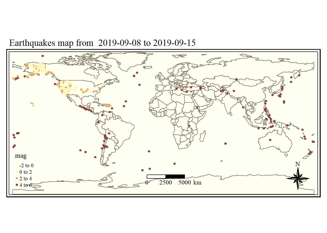
tmap Package

Let’s create a static map of the earthquake events using the tmap package. We will create a Simple Features object using the sf package. The Simple Features is an open standard developed and endorsed by the Open Geospatial Consortium (OGC), a not-for-profit organization. Simple Features is a hierarchical data model that represents a wide range of geometry types.

projcrs <- "+proj=longlat +datum=WGS84 +no_defs +ellps=WGS84 +towgs84=0,0,0"
title <- paste(
  "Earthquakes map from ",
  paste(
    as.Date(earthquakes$time[1]),
    as.Date(earthquakes$time[nrow(earthquakes)]
  ),
  sep = " to ")
)

df <- st_as_sf(
  x = earthquakes,
  coords = c("longitude", "latitude"),
  crs = projcrs
)

p <- tm_shape(spData::world) +
  tm_style("classic") +
  tm_fill(col = "white") +
  tm_borders() +
  tm_layout(main.title = title, main.title.size = 1.2) +
  tm_compass(type = "8star", position = c("right", "bottom"), size = 3) +
  tm_scale_bar(breaks = c(0, 2500, 5000), text.size = 0.8,
               position = c("left", "bottom")) +
  tm_shape(df) +
  tm_dots(size = 0.1, col = "mag", palette = "YlOrRd")
p

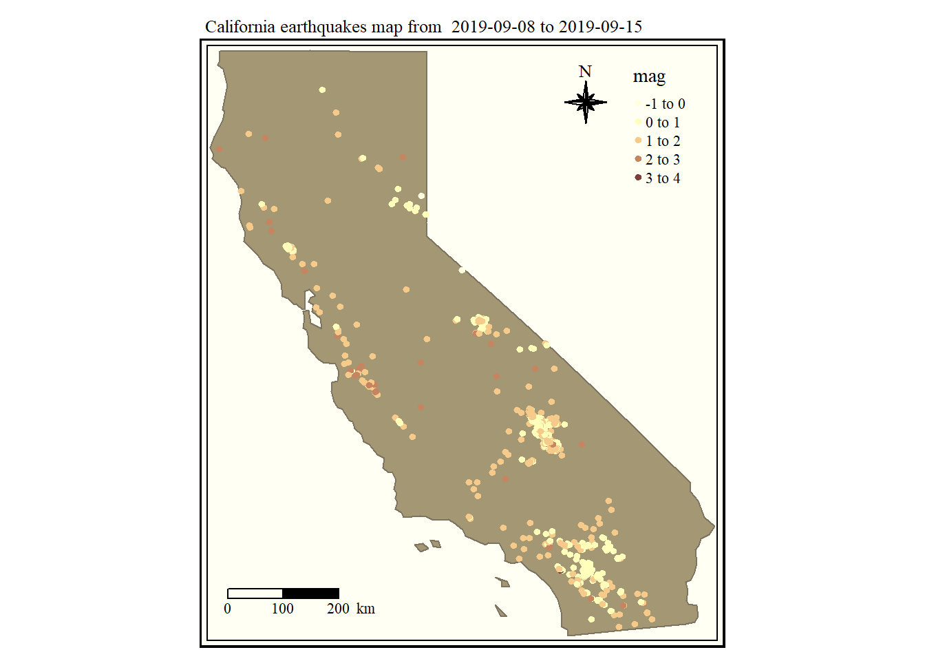
If we wish to create a map for a specific region, for instance California, we can use longitude and latitude to determine a rectangular geographical region that contains the California boundaries.

california_data <- earthquakes %>%
  filter(
    longitude >= -125 &
    longitude <= -114 &
    latitude <= 42.5 &
    latitude >= 32.5
  ) %>%
  droplevels()

map_california <- us_states %>%
  filter(NAME == "California")

df <- st_as_sf(
  x = california_data,
  coords = c("longitude", "latitude"),
  crs = st_crs(map_california)
)

p <- tm_shape(map_california) +
  tm_style("classic") +
  tm_fill(col = "palegreen4") +
  tm_borders() +
  tm_layout(main.title = paste("California earthquakes map from ",
            paste(as.Date(california_data$time[1]),
            as.Date(california_data$time[nrow(california_data)]),
            sep = " to ")), main.title.size = 0.8) +
  tm_compass(type = "8star", position = c("right", "top"), size = 2) +
  tm_scale_bar(breaks = c(0, 100, 200), text.size = 0.7,
               position = c("left", "bottom")) +
  tm_shape(df) +
  tm_dots(size = 0.1, col = "mag", palette = "YlOrRd")
p

A better approach is performing an inner join between the earthquake dataset and the map of California to determine the earthquakes within the California boundaries.

df <- st_as_sf(
  x = earthquakes,
  coords = c("longitude", "latitude"),
  crs = st_crs(map_california)
)
df_map_inner_join <- st_join(df, map_california, left = FALSE)

p <- tm_shape(map_california) +
  tm_style("classic") +
  tm_fill(col = "palegreen4") +
  tm_borders() +
  tm_layout(main.title = paste("California earthquakes map from ",
            paste(as.Date(california_data$time[1]),
            as.Date(california_data$time[nrow(california_data)]),
            sep = " to ")), main.title.size = 0.8) +
  tm_compass(type = "8star", position = c("right", "top"), size = 2) +
  tm_scale_bar(breaks = c(0, 100, 200), text.size = 0.7,
               position = c("left", "bottom")) +
  tm_shape(df_map_inner_join) +
  tm_dots(size = 0.1, col = "mag", palette = "YlOrRd")
p

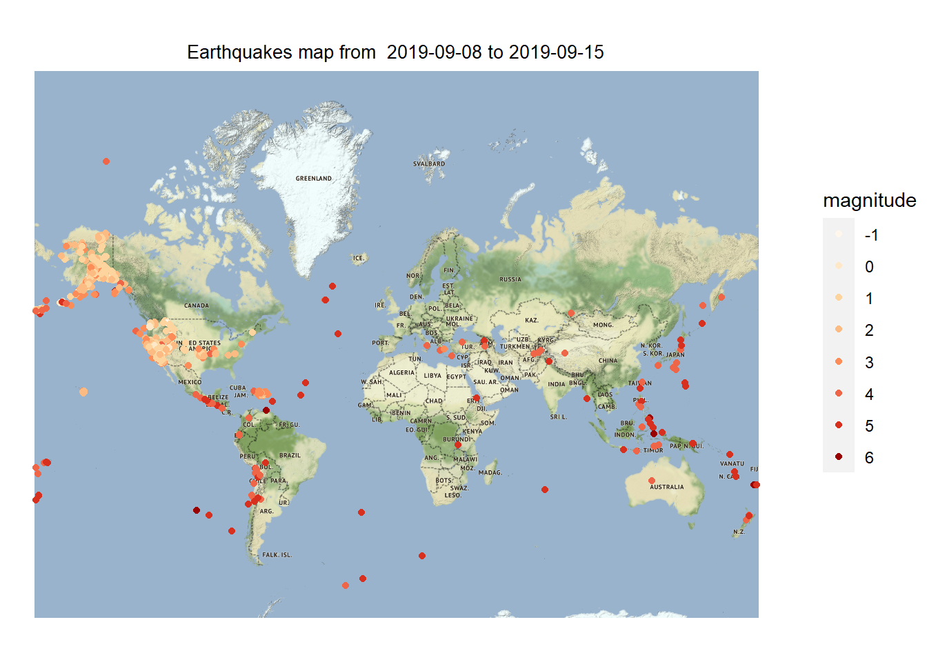
ggmap Package

Let’s create a static map of the earthquake events using the qmplot function within the ggmap package. Both qmplot and qmap are wrappers for a function called get_map that retrieves a base map layer. The qmplot function allows for the quick plotting of maps with data.

title <- paste(
  "Earthquakes map from ",
  paste(
    as.Date(earthquakes$time[1]),
    as.Date(earthquakes$time[nrow(earthquakes)]
  ),
  sep = " to ")
)

magnitude <- factor(round(earthquakes$mag))

suppressMessages(
  qmplot(x = longitude, y = latitude, data = earthquakes,
         geom = "point", color = magnitude,
         source = "stamen", zoom = 3) +
  scale_color_brewer(palette = 8) +
  ggtitle(title)) +
  theme(plot.title = element_text(margin = margin(b = -10), size = 10,
                                  hjust = 0.5, color = 'black'))

Layed Static Map

This example demonstrates that adding layers on a map created with ggplot2 is a relatively straightforward process, as long as the data is properly stored in a sf object.

Let’s use the classic dark-on-light theme for ggplot2 (theme_bw), which is more appropriate for geographic maps'

theme_set(theme_bw())

We will use the rnaturalearth package, which provides a map of countries of the entire world. We can use ne_countries function to pull country data and choose the scale. Note that rnaturalearthhires is necessary for scale equals “large”. The function can return sp classes by default or directly as defined in the argument returnclass.

world <- ne_countries(scale = "medium", returnclass = "sf")
class(world)

## [1] "sf"         "data.frame"

Let’s start by adding point data by defining two sites, according to their longitude and latitude, stored in a regular data.frame.

(sites <- data.frame(
  longitude = c(-80.144005, -80.109),
  latitude = c(26.479005, 26.83)
))

##   longitude latitude
## 1 -80.14401 26.47901
## 2 -80.10900 26.83000

Converting the data frame to a sf object allows sf to manage, on the fly, the coordinate system (both projection and extent). This can be useful if objects are not in the same projection. The projection (here WGS84, which is the CRS code #4326) must be defined in the sf object.

(sites <- st_as_sf(
  sites,
  coords = c("longitude", "latitude"), 
  crs = 4326, agr = "constant"
))

## Simple feature collection with 2 features and 0 fields
## Geometry type: POINT
## Dimension:     XY
## Bounding box:  xmin: -80.14401 ymin: 26.479 xmax: -80.109 ymax: 26.83
## Geodetic CRS:  WGS 84
##                     geometry
## 1 POINT (-80.14401 26.47901)
## 2      POINT (-80.109 26.83)

Now, let’s include state borders and names using the maps package. The maps package is automatically installed and loaded with ggplot2. First, we need to get the data.

# Get state data
states <- map('state', fill = TRUE, plot = FALSE) %>% st_as_sf()
head(states)

## Simple feature collection with 6 features and 1 field
## Geometry type: MULTIPOLYGON
## Dimension:     XY
## Bounding box:  xmin: -124.3834 ymin: 30.24071 xmax: -71.78015 ymax: 42.04937
## Geodetic CRS:  WGS 84
##            ID                           geom
## 1     alabama MULTIPOLYGON (((-87.46201 3...
## 2     arizona MULTIPOLYGON (((-114.6374 3...
## 3    arkansas MULTIPOLYGON (((-94.05103 3...
## 4  california MULTIPOLYGON (((-120.006 42...
## 5    colorado MULTIPOLYGON (((-102.0552 4...
## 6 connecticut MULTIPOLYGON (((-73.49902 4...

Next, we’re going to modify our state-level data to make some labels that we can add to the plot. There’s a few things we need to do. We need to change the state names (the ID variable) to title case. State names, which are not capitalized in the data from the maps package, can be changed to title case using the toTitleCase function in the tools package. We need to calculate the center of the state (where we want to add those state name labels), and add those centroid X and Y coordinates to the dataset. Centroids are computed with the st_centroid function, the coordinates extracted with the st_coordinates function (both from the sf package) and attached to the state object. Then, we need to add some “nudge” variables that will enable us to move the labels a little away from the centroid, as needed. Most of this will be accomplished using functions from the dplyr and sf packages.

# Change state name to title case
states <- states %>%
  mutate(ID = toTitleCase(ID))

# Add state centroids after turning off s2 processing to resolve spherical
# geometry failures
sf::sf_use_s2(FALSE)
states <- states %>% 
  mutate(centroid = st_centroid(geom))

# Add X and Y coordinates
states_coords <- states %>% 
  st_centroid() %>% 
  st_coordinates() %>%
  as_tibble()

# Add coordinates to states
states <- states %>%  
  bind_cols(states_coords) %>% 
  select(ID, X, Y, centroid, geom)

# Add nudge_y variable based on state name
states <- states %>% 
  mutate(
    nudge_y = case_when(
      ID == 'Florida' ~ 0.5,
      ID == 'South Carolina' ~ -1.5,
      TRUE ~ -1
    )
  ) 

County data also are available from the maps package, and can be retrieved with the same approach as for state data. We will only retain counties from Florida, and we will compute their area using st_area function from the sf package. We will use the area to fill in the counties to help identify the largest counties. For this, we will use the “viridis” colorblind-friendly palette, with some transparency.

counties <- st_as_sf(map("county", plot = FALSE, fill = TRUE))
counties <- subset(counties, grepl("florida", counties$ID))

# Turn off the s2 processing to resolve geometry failures
sf::sf_use_s2(FALSE)
counties$area <- as.numeric(st_area(counties))
head(counties)

## Simple feature collection with 6 features and 2 fields
## Geometry type: MULTIPOLYGON
## Dimension:     XY
## Bounding box:  xmin: -85.98951 ymin: 25.94926 xmax: -80.08804 ymax: 30.57303
## Geodetic CRS:  WGS 84
##                   ID                           geom       area
## 290  florida,alachua MULTIPOLYGON (((-82.66062 2... 2498863359
## 291    florida,baker MULTIPOLYGON (((-82.04182 3... 1542466064
## 292      florida,bay MULTIPOLYGON (((-85.40509 3... 1946587533
## 293 florida,bradford MULTIPOLYGON (((-82.4257 29...  818898090
## 294  florida,brevard MULTIPOLYGON (((-80.94747 2... 2189682999
## 295  florida,broward MULTIPOLYGON (((-80.89018 2... 3167386973

To make a more complete map of Florida, main cities will be added to the map. We first prepare a data frame with the five largest cities in the state of Florida, and their geographic coordinates.

flcities <- data.frame(
  state = rep("Florida", 5),
  city = c("Miami", "Tampa", "Orlando", "Jacksonville", "Sarasota"),
  lat = c(25.7616798, 27.950575, 28.5383355, 30.3321838, 27.3364347),
  lng = c(-80.1917902, -82.4571776, -81.3792365, -81.655651, -82.5306527)
)

We can now convert the data frame containing the coordinates to a sf format.

(flcities <- st_as_sf(
  flcities,
  coords = c("lng", "lat"), remove = FALSE, 
  crs = 4326, agr = "constant"
))

## Simple feature collection with 5 features and 4 fields
## Attribute-geometry relationship: 4 constant, 0 aggregate, 0 identity
## Geometry type: POINT
## Dimension:     XY
## Bounding box:  xmin: -82.53065 ymin: 25.76168 xmax: -80.19179 ymax: 30.33218
## Geodetic CRS:  WGS 84
##     state         city      lat       lng                   geometry
## 1 Florida        Miami 25.76168 -80.19179 POINT (-80.19179 25.76168)
## 2 Florida        Tampa 27.95058 -82.45718 POINT (-82.45718 27.95058)
## 3 Florida      Orlando 28.53834 -81.37924 POINT (-81.37924 28.53834)
## 4 Florida Jacksonville 30.33218 -81.65565 POINT (-81.65565 30.33218)
## 5 Florida     Sarasota 27.33643 -82.53065 POINT (-82.53065 27.33643)

To ensure that the names don’t overlap, we will use the geom_text_repel and geom_label_repel functions of the ggrepel package to deal with label placement, including automated movement of labels in case of overlap.

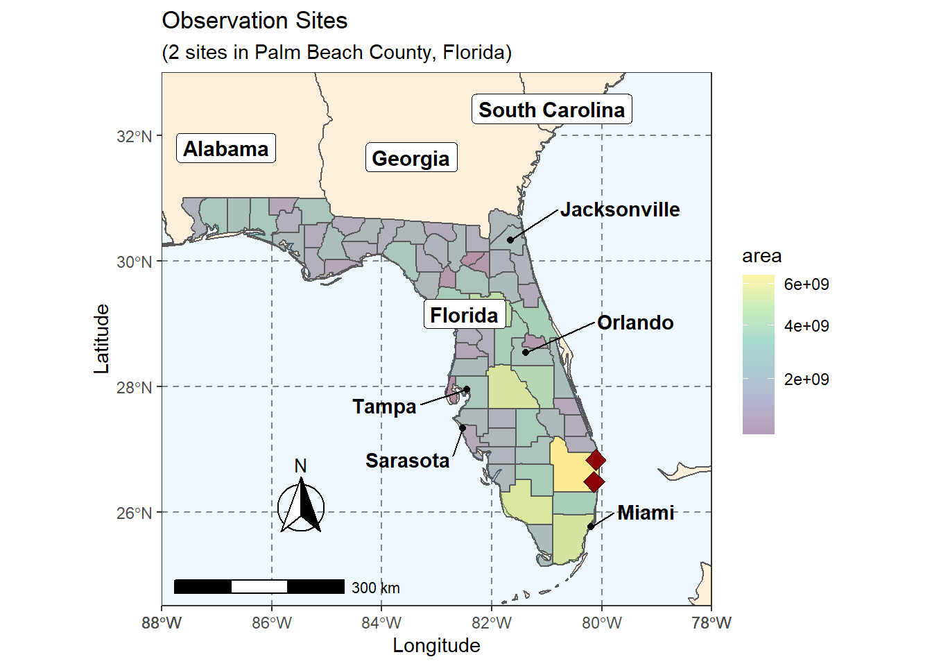
Finally, we can create the final map, with a general background map based on the world map, state and county delineations, state labels, main city names and locations, and a theme adjusted with titles, subtitles, axis labels, and a scale bar.

ggplot(data = world) +
  geom_sf(fill = "antiquewhite1") +
  geom_sf(data = counties, aes(fill = area)) +
  geom_sf(data = states, fill = NA) + 
  geom_sf(data = sites, size = 4, shape = 23, fill = "darkred") +
  geom_sf(data = flcities) +
  geom_text_repel(data = flcities, aes(x = lng, y = lat, label = city), 
                  fontface = "bold", nudge_x = c(1, -1.5, 2, 2, -1),
                  nudge_y = c(0.25, -0.25, 0.5, 0.5, -0.5)) +
  geom_label(data = states, aes(X, Y, label = ID), size = 4, fontface = "bold", 
             nudge_y = states$nudge_y) +
  scale_fill_viridis_c(trans = "sqrt", alpha = 0.4) +
  annotation_scale(location = "bl", width_hint = 0.4) +
  annotation_north_arrow(location = "bl", which_north = "true", 
                         pad_x = unit(0.75, "in"), pad_y = unit(0.5, "in"),
                         style = north_arrow_fancy_orienteering) +
  coord_sf(xlim = c(-88, -78), ylim = c(24.5, 33), expand = FALSE) +
  xlab("Longitude") + ylab("Latitude") +
  ggtitle("Observation Sites", subtitle = "(2 sites in Palm Beach County, Florida)") +
  theme(panel.grid.major = element_line(color = gray(0.5), linetype = "dashed", 
        size = 0.5), panel.background = element_rect(fill = "aliceblue"))