Introduction

Groundwater monitoring at landfills is essential for protecting environmental and public health by preventing contamination of aquifers. This involves the systematic examination of groundwater to enable early detection of any potential environmental releases. The detection monitoring process utilizes rigorous statistical analyses to differentiate between natural variations and those induced by landfill activities, thereby ensuring compliance with regulations.

Design of the detection monitoring program relies on two primary performance characteristics: sufficient statistical power and a low predetermined sitewide false positive rate (SWFPR). The SWFPR is assessed on a site-wide level and is distributed among the total number of annual statistical tests conducted. Fewer tests result in a lower single-test false negative error rate, and therefore an improvement in statistical power.

To illustrate this concept, the per-test false positive rate and the corresponding power for semiannual testing at four compliance wells will be calculated, first considering 10 constituents and then 100 constituents. This exercise aims to correct the misconception that increasing the number of constituents automatically enhances the statistical power of the detection monitoring program. The calculations will be performed using R version 4.4.2 (R Core Team 2024) and the EnvStats library (Millard 2013).

Background

Detection monitoring assumes that groundwater is clean or not impacted until shown otherwise. The main objective of detection monitoring is to determine if a statistically significant increase (SSI) greater than background concentrations have been observed; therefore, detection monitoring continues until an SSI over background is observed. The observed SSI must be large enough to account for the inherent uncertainty and variability in the data.

Groundwater monitoring regulations codified under 40 CFR Part 258 and 264 explicitly identify five basic formal statistical procedures for detection monitoring. These five procedures include:

• Parametric ANOVA followed by multiple comparisons procedures to identify statistically significant evidence of contamination.

• Nonparametric ANOVA based on the ranks of the data followed by multiple comparisons procedures to identify statistically significant evidence of contamination.

• A tolerance or prediction interval procedure in which an interval for each constituent is established from the distribution of the background data, and the level of each constituent in each compliance well is compared to the upper tolerance or prediction limit.

• A control chart approach that gives control limits for each constituent.

• Another statistical method that is approved by the Regional Administrator.

Among the statistical test procedures listed above, the United States Environmental Protection Agency (USEPA) (2009) recommends the use of simultaneous upper prediction limits (UPLs) for detection monitoring due to their established effectiveness in retesting strategies and their capability to specify an exact false positive error rate while preserving high statistical power. The mathematical foundations for retesting with prediction limits are well recognized, whereas the underpinnings for retesting using tolerance limits or control charts are less defined. In contrast to control charts, nonparametric prediction limits can be developed as an alternative to parametric prediction limits for data that display non-normality.

Prediction limits can be applied for both interwell and intrawell comparisons. For interwell comparisons, data from an upgradient monitoring well(s) serves as the background data set, while intrawell comparisons utilize background data from individual downgradient, compliance monitoring wells. At sites with inherent geochemical variations, notable differences between upgradient and downgradient wells could stem from spatial or hydrogeologic influences rather than the facility itself. In such cases, intrawell statistical approaches reduce the chances that spatial variability will impact the validity of the statistical tests.

Prediction Limits

Prediction limits provide flexible solutions for detection monitoring, allowing for minimal new measurements per compliance well and offering various statistical methods tailored to specific monitoring well networks and constituents. They can manage multiple statistical comparisons required by environmental regulations while controlling the false positive rate and ensuring adequate statistical power for effective monitoring and compliance.

Formally, prediction limits are constructed to contain one or more future observations or sample statistics generated from the background population with a specified probability equal to (1 - \(\alpha\)). The probability (1 - \(\alpha\)) is known as the confidence level of the limit. It represents the chance, over repeated applications of the limit to many similar data sets, that the prediction limit will contain future observations or statistics drawn from its background population.

A prediction limit based on normal or transformably normal populations is given by \(\overline{x} + \kappa s\) where \(\overline{x}\) is the background mean, s is the background standard deviation, and \(\kappa\) is a multiplier depending on the type of prediction limit under construction. The \(\kappa\)-multiplier is selected to account not only for the number of future comparisons, but also for the rules of the comparison strategy and the number of simultaneous tests to be conducted (e.g., the number of monitoring constituents times the number of compliance wells).

The prediction limit is then compared to one or more observations from a compliance point population. The acceptable range of concentrations includes all values no greater than the prediction limit. The appropriate prediction interval will generally have the form [0, UPL], with the UPL as the comparison of importance. Unless pH or a similar parameter is being monitored, a one-sided UPL is used in detection monitoring.

False Positive Rate

The primary objective of detection monitoring is to accurately identify actual groundwater contamination while minimizing false positive errors. This is challenging due to the inherent trade-off between statistical power (ability to detect true releases) and the likelihood of false positives. As facilities test multiple constituents semi-annually at several different compliance wells, the risk of false positives increases substantially with the number of tests conducted.

To manage cumulative false positive rates, three main strategies can be employed:

• Reduce the Number of Tests: Focus statistics on the most reliable indicators of a poential release to limit unnecessary testing, thereby reducing the overall false positive rate while improving the power of individual tests.

• Lower Individual Test False Positive Rates: Use methods like the Bonferroni adjustment to decrease the significance level for each test based on the number of tests. This reduces the chance of false positives but may lower the statistical power of detecting an actual release, if one occurs.

• Change Statistical Tests: Adopt different statistical methodologies that may better balance cumulative error rates and detection power based on the specific data and goals.

A target cumulative sitewide false positive rate (SWFPR) is set for effective monitoring, commonly recommended at 10% over a year (USEPA 2009). The SWFPR false positive rate is measured on a site-wide basis, partitioned among the total number of annual statistical tests. The total number of annual statistical tests used in SWFPR calculations depends on the number of valid monitoring constituents, compliance wells, and evaluation periods per year. Retesting strategies, such as the 1-of-m approach introduced by Davis and McNichols in 1987, allow for further sampling if initial results indicate potential contamination, helping to manage the SWFPR. If the initial test is within acceptable limits, no further samples are needed. However, if the initial value exceeds the background limit, additional sampling is required. A 1-of-3 plan allows for up to three measurements at each well, including the initial and two resamples, all of which must be statistically independent. Practical limitations exist regarding the number of independent samples and retests that can be conducted. Consequently, it is important to limit statitical parameters to those deemed reliable indicators of contamination to balance the risks of false positives and negatives effectively.

Statistical Power

Statistical power refers to the ability of a test to identify real increases in concentration levels above background (true SSIs). Power is reported as a fraction between 0 and 1, representing the probability that the test will identify a specific level or degree of increase above background. Statistical power varies with the size of the average population concentration above background, generally fairly low power to detect small incremental increases in concentrations and substantially higher power to detect larger incremental increases in concentrations.

While retesting strategies can help in limiting the SWFPR and ensure adequate statistical power, there are practical limits to meeting these goals due to the limited number of groundwater observations that can be collected and/or the number of retests which can feasibly be run. To balance the risks of false positive and false negative errors, the number of statistically-tested monitoring parameters should be limited to constituents thought to be reliable indicators of a contaminant release.

Chemicals that do not occur naturally, such as volatile organic compounds (VOCs) and semi-volatile organic compounds (SVOCs), are frequently used as indicators of groundwater contamination and are therefore included in monitoring programs. There is a common misconception that analyzing a greater number of these compounds enhances the statistical power of the detection monitoring program. However, incorporating a large number of VOCs and/or SVOCs can be counterproductive to maintaining adequate statistical power for the site as a whole. Consequently, it is recommended to select a limited number of reliable monitoring constituents, typically around 10 to 15, based on specific site requirements to ensure effective detection of a release, if it occurs. An excessive number of constituents can undermine the overall statistical effectiveness of a detection monitoring program (USEPA 2009).

The SWFPR is measured on a site-wide basis and partitioned among the total number of annual statistical tests. The total number of statistical tests depends on the number of monitoring constituents, compliance wells, and periodic evaluations. Fewer tests imply a lower single-test false negative error rate, and therefore an improvement in statistical power. For example, suppose 100 constituents are to be tested semiannually at four compliance wells totaling 800 annual statistical tests. The cumulative false positive error rate \(\alpha_{cum}\) is calculated as the probability of at least one statistically significant outcome for a total number of tests \(n_T\) in a calendar year at a single false positive error rate \(\alpha_{test}\). Using the properties of the Binomial distribution, this can be expressed as:

$$\alpha_{cum} = 1 - (1 - \alpha_{test})^{n_T}$$

By rearranging to solve for \(\alpha_{test}\) and substituting the 10% design SWFPR for \(\alpha_{cum}\), the needed per-test false positive error rate is calculated as:

$$\alpha_{test} = 1 - (0.9)^{1/n_T}$$

For 100 constituents, the per-test false positive rate would need to be set at \(\alpha_{test}\) = 0.000132 to maintain a 10% cumulative annual SWFPR. If only 10 constituents were selected for formal testing, the per-test rate would be increased to \(\alpha_{test}\) = 0.00132. For intrawell tests in which each monitoring well is compared to its own background data, USEPA (2009) suggests using a per well-constituent pair false positive rate (\(\alpha_{wc}\)). The \(\alpha_{wc}\) is 0.000263 for 100 constituents and 0.00263 for 10 constituents. For prediction limits and other detection monitoring tests, higher false positive test rates translate to lower \(\kappa\)-multipliers and improved statistical power.

The USEPA (2009) advises that the design of any statistical program for detection monitoring should fulfill the power standards outlined in the Unified Guidance. According to these guidelines, any statistical test must achieve a minimum of 55% to 60% annual power for detecting a 3 standard deviation increase above the true background mean, and at least 80% to 85% annual power for identifying a 4 standard deviation increase. A statistical test is deemed insufficient unless its power meets or surpasses the established minimum requirements for mean-level increases of 3 to 4 standard deviations.

Let’s determine the statistical power for the aforementioned example: four compliance wells tested semiannually for 10 constituents compared to 100 constituents. We’ll assume that intrawell testing is necessary due to statistically significant spatial variability observed across the monitoring well network. Additionally, let’s consider that the background sample size is eight.

Now, let’s load the necessary libraries and define the values for the detection monitoring variables, which include:

• nb = number of backgound samples
• nc = number of constituents
• nw = number of compliance wells
• r = number of future sampling events per year
• m = value of m for k-of-m retesting strategy
• swfpr = targeted sitewide false positive rate, by default set to 10%

First, we will evaluate the per well-constituent pair false positive rate, the \(\kappa\)-multiplier, and the power for 10 constituents. Thus, we will set the variable nc = 10.

# Load libraries
library(dplyr)
library(ggplot2)
library(patchwork)
library(EnvStats)

# Load function for creating plot showing power curve(s)
source('functions/power_curve.R')

# Set detection monitoring variables
nb <- 8
nc <- 10
nw <- 4
r <- 2
m <- 2
swfpr <- 0.1

# Turn off scientific notation
options(scipen = 999)

The target per well-constituent pair false positive rate and the \(\kappa\)-multiplier for 10 constituents is calculated below.

# Calculate target per well-constituent pair false positive rate
conf.intra <- (1 - swfpr)^(1/(nc*nw))  # intrawell testing

# Calculate alpha
(alpha.intra <- 1 - conf.intra)
## [1] 0.002630547

# Calculate the k-multiplier
K.intra <- predIntNormSimultaneousK(
  n = nb, k = 1, m = m, r = r,
  rule = "k.of.m",
  pi.type = "upper",
  n.mean = 1, 
  conf.level = conf.intra
)
round(K.intra, 2)
## [1] 2.85

For 10 constituents, the false positive rate for each well-constituent pair is 0.00263 and the \(\kappa\)-multiplier is 2.85.

The power is calculated using the predIntNormSimultaneousTestPower() function from the EnvStats library. The delta.over.sigma argument represents the difference between the mean of the population that was sampled to construct the prediction interval, and the mean of the population that will be sampled to produce the future observations (i.e., the number of standard deviations above the true background mean). Power will be calculated for both a 1-of-2 and a 1-of-3 retesting strategy.

#  Calculate the power for 1-of-2
pow.intra2 <- predIntNormSimultaneousTestPower(
  n = nb,  k = 1, m = 2, r = r,
  rule = 'k.of.m',
  delta.over.sigma = seq(0, 5, by = 0.1),  
  pi.type = 'upper',
  conf.level = conf.intra
)

#  Calculate the power for 1-of-3
pow.intra3 <- predIntNormSimultaneousTestPower(
  n = nb,  k = 1, m = 3, r = r,
  rule = 'k.of.m',
  delta.over.sigma = seq(0, 5, by = 0.1),  
  pi.type = 'upper',
  conf.level = conf.intra
)

# Create data frame to hold power estimates
dat <- data.frame(
  x = rep(seq(0, 5, by = 0.1), 2),
  y = c(pow.intra2, pow.intra3),
  type = c(rep('1-of-2', 51), rep('1-of-3', 51))
)

Now, let’s plot the power curves for 10 constituents and the two retesting strategies.

# Create plot showing power curve for 1-of-2 retesting strategy
p1 <- power_curve(
  dd = dat,
  test = '1-of-2',
  nb = nb, nw = nw,
  nc = nc, r = r
)

# Create plot showing power curve for 1-of-3 retesting strategy
p2 <- power_curve(
  dd = dat,
  test = '1-of-3',
  nb = nb, nw = nw,
  nc = nc, r = r
)

# Show plots
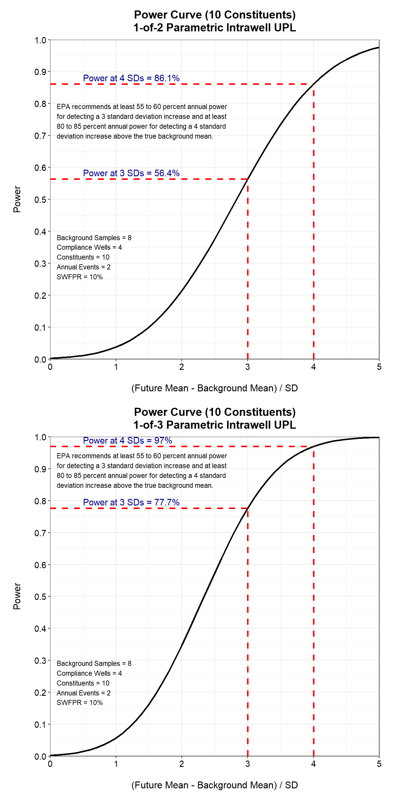
wrap_plots(p1, p2, ncol = 1)

For 10 constituents, both the 1-of-2 and 1-of-3 retesting strategies achieve the minimum power requirements outlined in the Unified Guidance (USEPA 2009) and are suitable for confirming that an apparent detection exceeds background. The per-test false positive rate is achieved based on how parametric prediction limits are developed.

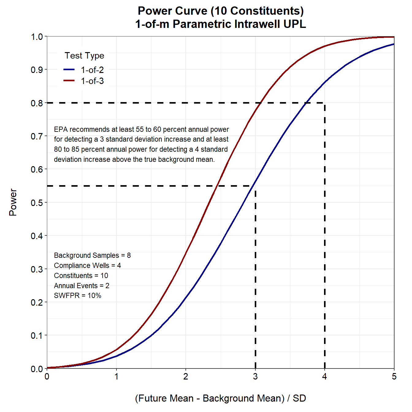
Let’s compare the power curves for the two retesting strategies, assuming 10 constituents. Dashed lines are used to identify the minimum power requirements of 55% annual power for detecting a 3 standard deviation increase and at least 80% annual power for identifying a 4 standard deviation increase above the true background mean.

# Create plot showing power curve for 1-of-2 retesting strategy
power_curve(
  dd = dat,
  test = 'both',
  nb = nb, nw = nw,
  nc = nc, r = r
)

Because the 1-of-2 retesting strategy achieves the minimum power requirements, there is no need to consider 1-of-3 retesting.

Now, let’s calculate the target per well-constituent pair false positive rate and the \(\kappa\)-multiplier for 100 constituents.

# Set number of constituents to 100
nc <- 100

# Calculate target per well-constituent pair false positive rate
conf.intra <- (1 - swfpr)^(1/(nc*nw))  # intrawell testing

# Calculate alpha
(alpha.intra <- 1 - conf.intra)
## [1] 0.0002633666

# Calculate the k-multiplier
K.intra <- predIntNormSimultaneousK(
  n = nb, k = 1, m = m, r = r,
  rule = "k.of.m",
  pi.type = "upper",
  n.mean = 1, 
  conf.level = conf.intra
)
round(K.intra, 2)
## [1] 4.34

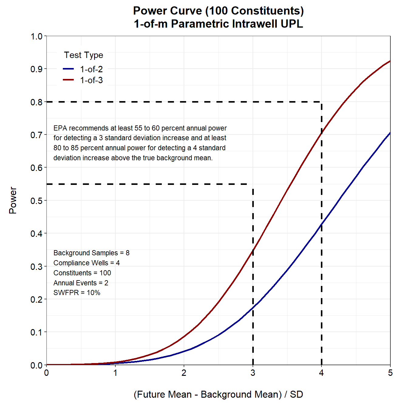
For 100 constituents, the false positive rate for each well-constituent pair is 0.000263 and the \(\kappa\)-multiplier is 4.34. The \(\kappa\)-multiplier is approximately 50% higher than the multiplier for 10 constituents. While this adjustment lowers the per-test false positive rate, it simultaneously diminishes the detection monitoring program’s ability to identify a release if one occurs. This is illustrated below in the power curves for 100 constituents using the 1-of-2 and 1-of-3 retesting strategies.

#  Calculate the power for 1-of-2
pow.intra2 <- predIntNormSimultaneousTestPower(
  n = nb,  k = 1, m = 2, r = r,
  rule = 'k.of.m',
  delta.over.sigma = seq(0, 5, by = 0.1),  
  pi.type = 'upper',
  conf.level = conf.intra
)

#  Calculate the power for 1-of-3
pow.intra3 <- predIntNormSimultaneousTestPower(
  n = nb,  k = 1, m = 3, r = r,
  rule = 'k.of.m',
  delta.over.sigma = seq(0, 5, by = 0.1),  
  pi.type = 'upper',
  conf.level = conf.intra
)

# Create data frame to hold power estimates
dat <- data.frame(
  x = rep(seq(0, 5, by = 0.1), 2),
  y = c(pow.intra2, pow.intra3),
  type = c(rep('1-of-2', 51), rep('1-of-3', 51))
)

# Create plot showing power curve for 1-of-2 retesting strategy
p1 <- power_curve(
  dd = dat,
  test = '1-of-2',
  nb = nb, nw = nw,
  nc = nc, r = r
)

# Create plot showing power curve for 1-of-3 retesting strategy
p2 <- power_curve(
  dd = dat,
  test = '1-of-3',
  nb = nb, nw = nw,
  nc = nc, r = r
)

# Show plots
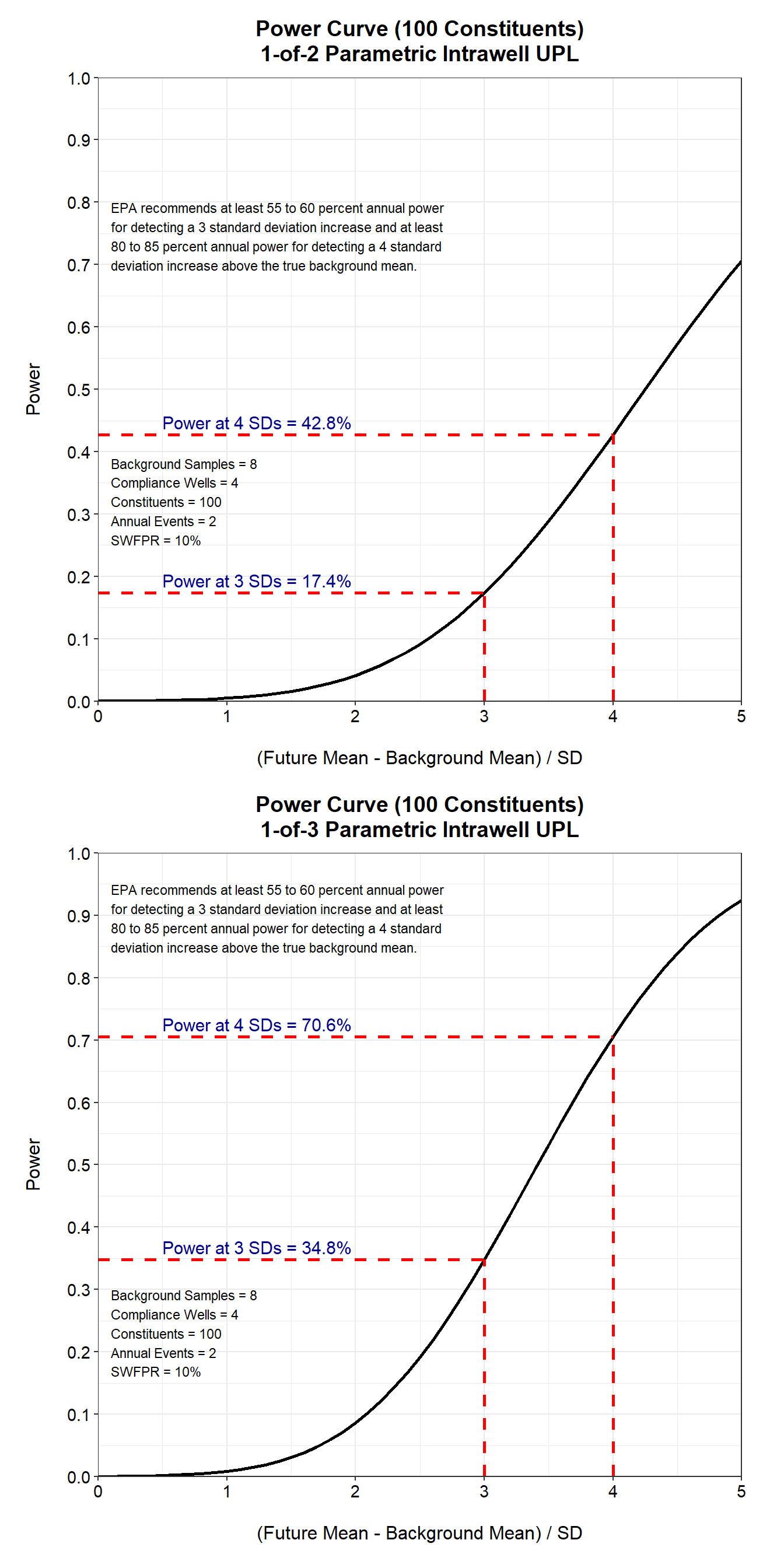
wrap_plots(p1, p2, ncol = 1)

For 100 constituents, neither the 1-of-2 nor the 1-of-3 retesting strategies achieve the minimum required power requirements outlined in the Unified Guidance (USEPA 2009). As currently designed, the detection monitoring program would not be suitable to verify that an apparent detection exceeds background. This is clearly illustrated in the power curves for both retesting strategies displayed below. The power of the 1-of-2 retesting strategy is extremely low, while the power of the 1-of-3 retesting strategy shows slight improvement, yet still falls short of the minimum requirements.

# Create plot showing power curve for 1-of-2 retesting strategy
power_curve(
  dd = dat,
  test = 'both',
  nb = nb, nw = nw,
  nc = nc, r = r
)

Conclusions

Detection monitoring at landfills uses robust statistical analyses to distinguish between natural variations in groundwater and those caused by landfill activities, ensuring regulatory compliance. Simultaneous UPLs are recommended for their effectiveness in retesting strategies, maintaining an exact false positive error rate while achieving strong statistical power. This is critical in environmental monitoring, which often involve numerous statistical comparisons that can inflate the overall false positive rate.

Design of the detection monitoring program is centered on two key performance characteristics: adequate statistical power and a low predetermined SWFPR. The SWFPR is assessed site-wide and is distributed among the total annual tests, which depends on the number of monitoring constituents, compliance wells, and periodic evaluations. Fewer tests result in a lower single-test false negative error rate, and therefore an improvement in statistical power.

Retesting strategies help manage the SWFPR but there are practical constraints on the number of groundwater observations that can be collected and/or the number of retests which can feasibly be run. To effectively balance false positive and negative rates, the number of statistically-tested monitoring parameters should be limited to constituents thought to be reliable indicators of a contaminant release. Generally, 10 to 15 constituents are selected based on specific site requirements to ensure effective detection of contamination.

Statistically analyzing too many constituents can undermine the overall statistical effectiveness of a detection monitoring program. Thus, a focused monitoring program that prioritizes a small number of carefully selected constituents, likely influenced by landfill leachate, improves the power of detection monitoring, enhancing the chances of accurately identifying true contamination while minimizing unnecessary investigations.

References

Davis C.B. and R.J. McNichols. 1987. One-sided intervals for at least p of m observations from a normal population on each of r future occasions. Technometrics, 29, 359-370.

Millard, S.P. EnvStats: An R Package for Environmental Statistics. Springer, NY.

R Core Team. 2024. R: A Language and Environment for Statistical Computing. R Foundation for Statistical Computing, Vienna, Austria. https://www.R-project.org.

United States Environmental Protection Agency (USEPA). 2009. Statistical Analysis of Groundwater Monitoring Data at RCRA Facilities: Unified Guidance. EPA-530-R-09-007. Office of Resource Conservation and Recovery, U.S. Environmental Protection Agency. March.