Introduction

Real data often contain observations that behave differently from the majority. Such data points are called anomalies in machine learning, and outliers in statistics. Outliers may be caused by errors, but they can also represent values recorded under exceptional circumstances, or that belong to another population. It is important to be able to detect outliers, which may (a) bias interpretations and conclusions drawn from the data, or (b) contain valuable nuggets of information. The different approaches for handling outliers can drastically change the interpretation of the data. Therefore, adequate treatment of outliers is crucial for conducting efficient and accurate data analysis.

In practice, one often tries to detect outliers using diagnostics starting from a classical univariate approach. One method is Dixon’s Outlier Test (Dixon 1953). Dixon’s test is recommended by the U.S. Environmental Protection Agency (2009) for outlier identification during the statistical analysis of groundwater monitoring data. The test is designed for cases where there is only a single high or low outlier, although it can be adapted to test for multiple outliers. Classical methods, such as Dixon’s test, can be affected by outliers so strongly that they may not detect anomalous observations (called masking), or may identify good data as outliers (known as swamping). Robust statistics, including multivariate analyses, can be used to identify outliers while avoiding these effects. However, this factsheet will explore outlier identification using Dixon’s Outlier Test.

Outliers

A common problem in data analysis is dealing with outliers in a set of data. In statistics, an outlier is an observation point that is distant from other observations. An outlier may be due to variability in the measurement or it may indicate an erroneous result; the latter are generally excluded from the data prior to analyses. When multiple outliers are present in the data, the evaluation becomes more complicated. One problem is that one outlier may mask another outlier in a single outlier test. When evaluating a dataset for outliers, two questions usually arise:

• Is the value in question truly an outlier?
• Can I eliminate the value and proceed with the data analysis?

Statistical methods are available to identify observations that appear to be rare or unlikely given the available data. However, this does not mean that the values identified as statistical outliers should always be removed. It is essential to understand the effect outliers have on your data interpretation and analysis. As an illustration, let’s compare the fit of a simple linear regression model on a dataset with and without outliers. First, let’s load some data and inject outliers into the original data.

# Load data
cars1 <- cars[1:30, ]

# Create outliers
outliers <- data.frame(
  speed = c(19, 19, 20, 20, 20),
  dist = c(190, 186, 210, 220, 218)
)

# Add outliers to original data
cars2 <- rbind(cars1, outliers)
str(cars2)

## 'data.frame':	35 obs. of  2 variables:
##  $ speed: num  4 4 7 7 8 9 10 10 10 11 ...
##  $ dist : num  2 10 4 22 16 10 18 26 34 17 ...

Now that we have a dataset containng outliers, let’s plot the data with a linear regression model.

# Plot data with outliers
par(mfrow = c(1, 2))
plot(
  cars2$speed, cars2$dist,
  xlim = c(0, 28), ylim = c(0, 230),
  main = "With Outliers",
  xlab = "speed", ylab = "dist", pch = 16,
  col = "black", cex = 1
)
abline(lm(dist ~ speed, data = cars2), col = "blue", lwd = 3, lty = 2)

# Plot of original data without outliers
plot(
  cars1$speed, cars1$dist,
  xlim = c(0, 28), ylim = c(0, 230),
  main = "Outliers Removed", xlab = "speed", ylab = "dist", pch = 16,
  col = "black", cex = 1
)
abline(lm(dist ~ speed, data = cars1), col = "blue", lwd = 3, lty = 2)

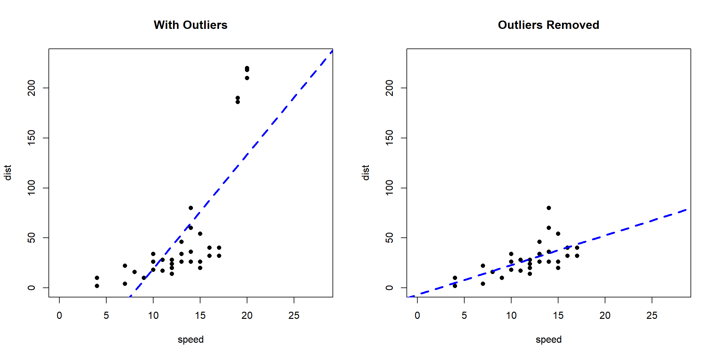
After removing the outliers, there is a significant change in slope of the best fit line. Predictions made when the outliers are included in the dataset would be exaggerated (high error) for larger values of speed because of the larger slope.

Prior to conducting a statistical evaluation for outliers, the first step is to visualize the data. Graphical displays provide added insight into the data that are not possible to visualize and understand by reviewing test statistics. Plotting methods should include scatterplots, box-and-whisker plots, histograms, and probability plots. These graphical presentations of the data show the central tendency, degree of symmetry, range of variation, and potential outliers of a dataset.

Dixon’s Outlier Test

Dixon’s test is valid for data sets with up to 25 observations and is designed to detect a single outlier in a dataset. The test falls in the general class of tests for discordancy (Barnett and Lewis 1994). The test statistic for such procedures is generally a ratio: the numerator is the difference between the suspected outlier and some summary statistic of the data set, while the denominator is always a measure of spread within the data. Dixon’s test assumes that the data values (aside from those being tested as potential outliers) are normally distributed. Because environmental data tend to be right-skewed, a test that relies on an assumption of a normal distribution may identify a relatively large number of statistical outliers.

For testing the largest sample observation \((X_k)\) to be an outlier, the sample is ordered in ascending order:

$$X_1 \le X_2 \le ... \le X_k$$

Dixon’s test is concerned with only the first or the last of the differences in this ordered set:

$$W_1 = X_2 - X_1 \quad or \quad W_{k-1} = X_k - X_{k-1}$$

Dixon’s Q statistic is the larger of the two differences above divided by the range of the k values \((X_k - X_1)\):

$$Q = the \ larger \ of \ \frac{w_1}{(X_k - X_1} \quad and \quad \frac{w_{k-1}}{(X_k - X_1)}$$

When Q exceeds the appropriate critical value then the corresponding extreme value, either \(X_1\) or \(X_k\), is said to be an outlier. The critical values for Q depend upon both the number of values in the original dataset, k, and the significance level of the test.

As an illustration, let’s apply Dixon’s test to a dataset containing two extreme values. Prior to running Dixon’s test, let’s visualize the data using a simple dot chart.

# Create data
x <- c(
 19, 21, 25, 30, 33,
 36, 41, 44, 48, 50,
 53, 55, 89, 90
)

# Make dot chart of data
library(BHH2)
dotPlot(x)
mean.x <- mean(x)
sd.x   <- sd(x)
lines(rep(mean.x         , 2), c(0.2, 0.25)) # Vertical line at mean
lines(rep(mean.x + 2*sd.x, 2), c(0.2, 0.25)) # Vertical line at mean + 2 SD
text(mean.x         , 0.3, expression(bar(x)))
text(mean.x + 2*sd.x, 0.3, expression(paste(bar(x), " + 2s")))

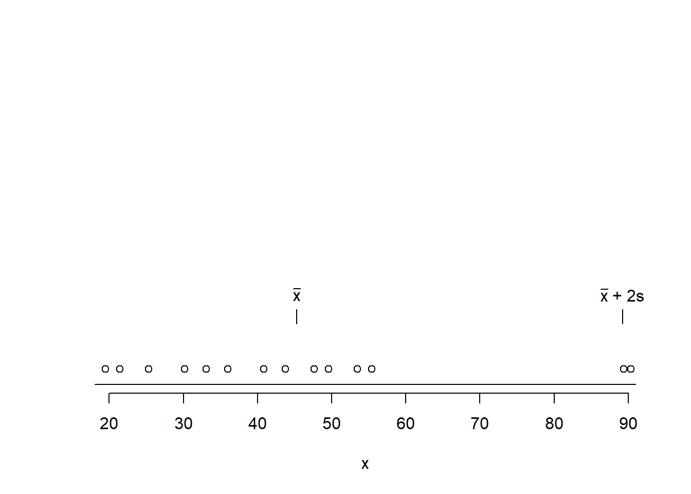
The dot chart indicates that values 89 and 90 are located distant from the other observations. Let’s apply Dixon’s test to the data.

library(outliers)
dixon.test(x, type = 0, opposite = FALSE, two.sided = TRUE)

## 
## 	Dixon test for outliers
## 
## data:  x
## Q = 0.53846, p-value = 0.1114
## alternative hypothesis: highest value 90 is an outlier

Dixon’s test gives a p-value of 0.111, indicating the value of 90 is not an outlier at a significance level of 0.10, corresponding to a confidence level of 90%. Let’s rerun Dixon’s test when excluding 90 from the dataset.

library(outliers)
dixon.test(x[-length(x)], type = 0, opposite = FALSE, two.sided = TRUE)

## 
## 	Dixon test for outliers
## 
## data:  x[-length(x)]
## Q = 0.52941, p-value = 0.0884
## alternative hypothesis: highest value 89 is an outlier

Now the p-value is 0.088, indicating the value of 89 is an outlier at a significance level of 0.10. Because 89 is considered an outlier, any value greater than 89 (such as 90) also would be considered an outlier.

Measurement Continuum Issue

Dixon’s test is simple, easy to understand, and is widely used in the scientific community. The critical values for Dixon’s test are obtained under the assumption that the values in the dataset are all points from a continuum. That is, the computations assume that each value is known to many decimal places. In practice this is seldom the case. Often the data are rounded to some small number of digits. Because data are recorded to some specific measurement increment, this can become a problem for Dixon’s test. For example, let’s apply Dixon’s test to a simple dataset consisting of three values that are extremely homogeneous.

x <- c(323.2, 323.2, 323.3)
dixon.test(x, opposite = FALSE, two.sided = TRUE)

## 
## 	Dixon test for outliers
## 
## data:  x
## Q = 1, p-value < 2.2e-16
## alternative hypothesis: highest value 323.3 is an outlier

Dixon’s test tells us that the value of 323.3 is an outlier at a significance level of 0.01, corresponding to a confidence level of 99%! Of course, this result makes no sense for these three observations.

The problem with using Dixon’s test is that the possible values for the test statistic depends upon how many measurement increments are contained in the range of the data. In the example above, the smallest and largest values differed by only one measurement increment (one-tenth of a unit). For Dixon’s test to work as intended, the possible values for the test statistic must form a reasonable continuum between zero and one. When the range of the data only represents a handful of measurement increments, this condition will not be satisfied, and the actual significance level of the test can be considerably different from the design significance level.

Conclusion

Data recorded to some specific measurement increment can become a problem for outlier tests, such as Dixon’s test. To use Dixon’s test, you should have a large number of measurement increments between the minimum and maximum of your data. Additionally, Dixon’s test assumes that the data values (aside from those being tested as potential outliers) are normally distributed. Most sample distributions are not normally distributed. It is important to note that statistical outliers may actually be part of the normal population of the data. Outlying observations should not be removed from a dataset based soley on a statistical test. There should be a scientific explanation or quality assurance basis justifying omitting the data.

References

Barnett V. and T. Lewis. 1994. Outliers in Statistical Data, 3rd Edition. New York: John Wiley & Sons.

Dixon W.J. 1953. Processing Data for Outliers. J. Biometrics 9, 74-89.

U.S. Environmental Protection Agency (USEPA). 2009. Statistical Analysis of Groundwater Monitoring Data at RCRA Facilities-Unified Guidance. EPA 530/R-09-007. Office of Research and Development. March.