Feature Selection Methods for Machine Learning
By Charles Holbert
February 14, 2020
Introduction
Feature Selection is a core concept in machine (statistical) learning that can have significant impacts on model performance. Feature Selection (also referred to as variable selection) is the process by which you select those features which contribute most to your prediction variable or output. The data features that are used to train a model have a large influence on the performance of that model; irrelevant or partially relevant features can negatively impact model performance. As such, feature selection and data cleaning are the first and most important steps of model design.
One of the primary reasons to measure the strength or relevance of the predictor variables is to filter which varaibles should be used as inputs in a model. In many data analyses and modeling projects, hundreds or even thousands of features are collected. From a practical perspective, a model with more features often becomes harder to interpret and is costly to compute. Some models are more resistant to non-informative predictors (e.g., the Lasso and tree-based methods) than others. As the number of attributes becomes large, exploratory analysis of all the predictors may be infeasible. Data driven feature selection can be useful when sifting through large amounts of data. Ranking predictors based on a quantitative relevance score is critical in creating an effective predictive model. Fewer attributes is desirable because it reduces the complexity of the model, and a simpler model is simpler to understand and explain.
Feature selection is different from dimensionality reduction. Both methods seek to reduce the number of attributes in the dataset, but a dimensionality reduction method does so by creating new combinations of attributes, whereas feature selection methods include and exclude attributes in the data without changing them. The objective of variable selection is three-fold: improving the prediction performance of the predictors, providing faster and more cost-effective predictors, and providing a better understanding of the underlying process that generated the data (Guyon and Elisseeff 2003).
This factsheet presents various methods that can be used to identify the most important predictor variables that explain the variance of the response variable. In this context, variable importance is taken to mean an overall quantification of the relationship between the predictor and outcome.
Data
To illustrate the concepts of feature selection, we will use the Ozone data from the mlbench package. The Ozone data contains daily ozone levels and meterorologic data in the Los Angeles basin during 1976. It is available as a data frame with 203 observations and 13 variables, where each observation represents one day.
Prior to jumping into the feature selection, let’s explore the data using a combination of summary statistics (means and medians, variances, and counts) and graphical presentations. First, let’s load and inspect the structure of the data.
# Read data
inputData <- read.csv(
  "./data/ozone1.csv",
  stringsAsFactors = FALSE,
  header = TRUE
)
str(inputData)
## 'data.frame':	203 obs. of  13 variables:
##  $ Month                : int  1 1 1 1 1 1 1 1 1 1 ...
##  $ Day_of_month         : int  5 6 7 8 9 12 13 14 15 16 ...
##  $ Day_of_week          : int  1 2 3 4 5 1 2 3 4 5 ...
##  $ ozone_reading        : num  5.34 5.77 3.69 3.89 5.76 6.39 4.73 4.35 3.94 7 ...
##  $ pressure_height      : int  5760 5720 5790 5790 5700 5720 5760 5780 5830 5870 ...
##  $ Wind_speed           : int  3 4 6 3 3 3 6 6 3 2 ...
##  $ Humidity             : int  51 69 19 25 73 44 33 19 19 19 ...
##  $ Temperature_Sandburg : int  54 35 45 55 41 51 51 54 58 61 ...
##  $ Temperature_ElMonte  : num  45.3 49.6 46.4 52.7 48 ...
##  $ Inversion_base_height: int  1450 1568 2631 554 2083 111 492 5000 1249 5000 ...
##  $ Pressure_gradient    : int  25 15 -33 -28 23 9 -44 -44 -53 -67 ...
##  $ Inversion_temperature: num  57 53.8 54.1 64.8 52.5 ...
##  $ Visibility           : int  60 60 100 250 120 150 40 200 250 200 ...
Let’s take a closer look at the data by creating summary statistics for each variable. This can be useful for identifying missingdata, if any at present.
summary(inputData)
##      Month         Day_of_month   Day_of_week    ozone_reading
##  Min.   : 1.000   Min.   : 1.0   Min.   :1.000   Min.   : 0.72
##  1st Qu.: 3.000   1st Qu.: 9.0   1st Qu.:2.000   1st Qu.: 4.77
##  Median : 6.000   Median :15.0   Median :3.000   Median : 8.90
##  Mean   : 6.522   Mean   :15.7   Mean   :3.005   Mean   :11.37
##  3rd Qu.:10.000   3rd Qu.:23.0   3rd Qu.:4.000   3rd Qu.:16.07
##  Max.   :12.000   Max.   :31.0   Max.   :5.000   Max.   :37.98
##  pressure_height   Wind_speed        Humidity     Temperature_Sandburg
##  Min.   :5320    Min.   : 0.000   Min.   :19.00   Min.   :25.00
##  1st Qu.:5690    1st Qu.: 3.000   1st Qu.:46.00   1st Qu.:51.50
##  Median :5760    Median : 5.000   Median :64.00   Median :61.00
##  Mean   :5746    Mean   : 4.867   Mean   :57.61   Mean   :61.11
##  3rd Qu.:5830    3rd Qu.: 6.000   3rd Qu.:73.00   3rd Qu.:71.00
##  Max.   :5950    Max.   :11.000   Max.   :93.00   Max.   :93.00
##  Temperature_ElMonte Inversion_base_height Pressure_gradient
##  Min.   :27.68       Min.   : 111          Min.   :-69.00
##  1st Qu.:49.64       1st Qu.: 869          1st Qu.:-14.00
##  Median :56.48       Median :2083          Median : 18.00
##  Mean   :56.54       Mean   :2602          Mean   : 14.43
##  3rd Qu.:66.20       3rd Qu.:5000          3rd Qu.: 43.00
##  Max.   :82.58       Max.   :5000          Max.   :107.00
##  Inversion_temperature   Visibility
##  Min.   :27.50         Min.   :  0.0
##  1st Qu.:51.26         1st Qu.: 60.0
##  Median :60.98         Median :100.0
##  Mean   :60.69         Mean   :122.2
##  3rd Qu.:70.88         3rd Qu.:150.0
##  Max.   :90.68         Max.   :350.0
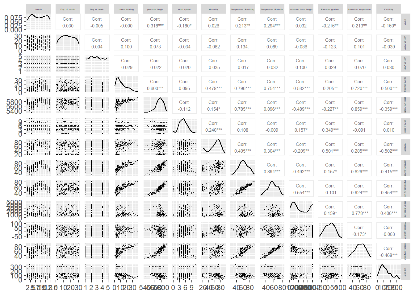
Graphical displays of the data provide added insight into data that are not possible to visualize and understand by reviewing summary statistics. Although some problems in the data can be identified by reviewing summary statistics, other problems are easier to find visually. Numerical reduction methods do not retain all the information contained in the data.
Let’s use the ggpairs function of the GGally package to build a scatterplot matrix. Scatterplots of each pair of numeric variable are drawn on the left part of the figure, the Spearman correlation coefficient is displayed on the right, and variable distribution is shown on the diagonal.
# Quick visual analysis of data
library(GGally)
ggpairs(
  data = inputData,
  upper = list(
    continuous = wrap("cor",
                      method = "spearman",
                      size = 2,
                      alignPercent = 1)
  ),
  lower = list(continuous = wrap("points", size = 0.1))
) +
theme(strip.text = element_text(size = 2.5))
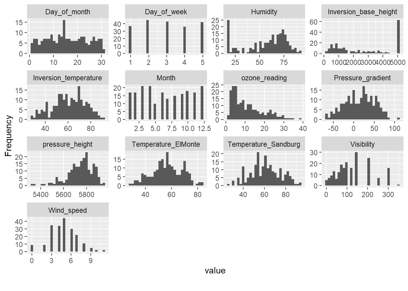
We can quickly inspect other aspects of the data using the DataExplorer package. The package is flexible with input data classes and can manage most any dataframe-like object.
# Plot histograms
DataExplorer::plot_histogram(inputData)
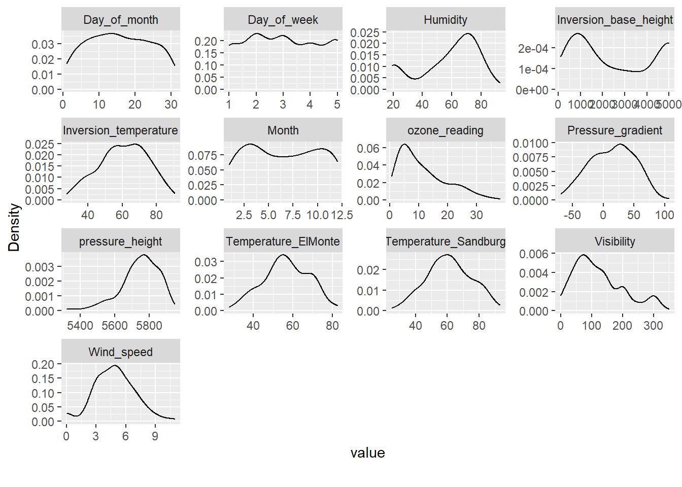
# Plot density
DataExplorer::plot_density(inputData)
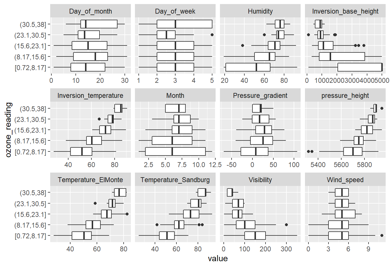
# Box plots
DataExplorer::plot_boxplot(inputData, by = 'ozone_reading',  ncol = 4)
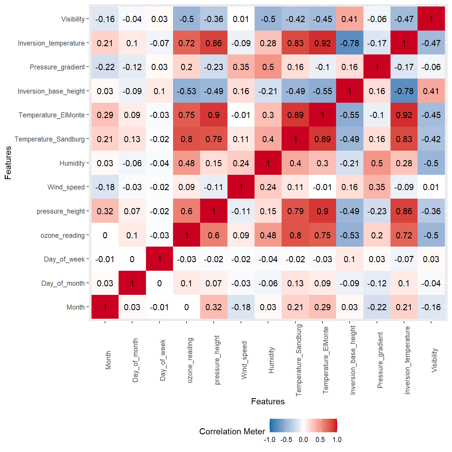
Let’s create a correlation heatmap to visually inspect the correlation between the varables. The colors of the heatmap correspond to the nonparametric Spearman’s rank-order correlation, which is used to measure the strength of a monotonic relationship between paired data. Whereas Pearson’s correlation evaluates the linear relationship between two continuous variables, Spearman’s correlation evaluates the monotonic relationship where the variables tend to change together, but not necessarily at a constant rate.
DataExplorer::plot_correlation(
  data = inputData,
  cor_args = list(method = 'spearman', use = 'complete.obs')
)
Now that we have examined the data, let’s move on to evaluating variable importance.
Variable Importance
Near Zero Variance
Zero variance variables only contain a single unique value and thus, provide no useful information to a model. Additionally, variables that have near-zero variance also offer very little, if any, information to a model. Furthermore, these variables can cause problems during resampling as there is a high probability that a given sample will only contain a single unique value (the dominant value) for that feature. A rule of thumb for detecting near-zero variance features is (Boehmke and Greenwell 2019):
- The fraction of unique values over the sample size is low (say
\(\leq\)10%). - The ratio of the frequency of the most prevalent value to the frequency of the second most prevalent value is large (say
\(\geq\)20%).
If both of these criteria are true then it is often advantageous to remove the variable from the model. For the Ozone data, we do not have any zero or near-zero variance variables.
# Find zero and near-zero variance variables using caret
library(caret)
preds <- colnames(inputData[, -grep("ozone_reading", colnames(inputData))])

nearZeroVar(x = inputData[, preds], saveMetrics = TRUE)
##                       freqRatio percentUnique zeroVar   nzv
## Month                  1.000000      5.911330   FALSE FALSE
## Day_of_month           1.000000     15.270936   FALSE FALSE
## Day_of_week            1.046512      2.463054   FALSE FALSE
## pressure_height        1.000000     23.645320   FALSE FALSE
## Wind_speed             1.257143      5.418719   FALSE FALSE
## Humidity               2.272727     29.556650   FALSE FALSE
## Temperature_Sandburg   1.125000     28.571429   FALSE FALSE
## Temperature_ElMonte    1.000000     67.487685   FALSE FALSE
## Inversion_base_height 15.750000     61.576355   FALSE FALSE
## Pressure_gradient      1.000000     52.216749   FALSE FALSE
## Inversion_temperature  1.000000     71.428571   FALSE FALSE
## Visibility             1.190476     11.330049   FALSE FALSE
Maximal Information Coefficient, Rank Correlation, and pseudo \(R^2\)
The maximal information coefficient (MIC) is a measure of two-variable dependence designed specifically for rapid exploration of many-dimensional data sets (Reshef et al. 2018). MIC is part of a larger family of maximal information-based nonparametric exploration (MINE) statistics, which can be used to identify important relationships in datasets (Reshef et al. 2016). The nonparametric Spearman’s rank correlation coefficient can be used to measure the relationship between each predictor and the outcome. A third metric uses a pseudo \(R^2\) statistic derived from the residuals of a locally weighted regression model (LOESS) fit to each predictor (Kuhn and Johnson 2016).
# Use apply function to estimate correlations between predictors and rate
corr_values <- apply(inputData[, preds],
                     MARGIN = 2,
                     FUN = function(x, y) cor(x, y,
                                              method = 'spearman'),
                     y = inputData[, "ozone_reading"])

# The caret function filterVarImp with the nonpara = TRUE option (for
# nonparametric regression) creates a LOESS model for each predictor
# and quantifies the relationship with the outcome.
library(caret)
loess_results <- filterVarImp(
  x = inputData[, preds],
  y = inputData[, "ozone_reading"],
  nonpara = TRUE
)

# The minerva package can be used to calculate the MIC statistics
# between the predictors and outcomes. The mine function computes
# several quantities including the MIC value.
library(minerva)
mine_values <- mine(
  inputData[, preds],
  inputData[, "ozone_reading"]
)

# Several statistics are calculated
names(mine_values)
## [1] "MIC" "MAS" "MEV" "MCN" "MICR2" "GMIC" "TIC"
mic_values <- cbind.data.frame(preds, round(mine_values$MIC, 4))

# Merge results
imout <- cbind.data.frame(
  mic_values,
  data.frame(corr_values),
  loess_results
)

colnames(imout) <- c('Variable', 'MIC', 'Corr', 'R2')
imout[order(-imout$MIC), -1]
##                          MIC         Corr          R2
## Temperature_Sandburg  0.5972  0.796290240 0.662406921
## Temperature_ElMonte   0.5600  0.753758794 0.668355181
## Inversion_temperature 0.5234  0.720327814 0.568031585
## Visibility            0.4063 -0.499758768 0.226853234
## Inversion_base_height 0.4061 -0.532412005 0.336852964
## pressure_height       0.3898  0.600408565 0.444451196
## Humidity              0.3447  0.478489867 0.242830771
## Month                 0.3315 -0.000260642 0.001951453
## Pressure_gradient     0.2658  0.204629227 0.170865783
## Day_of_month          0.2543  0.099574829 0.006995751
## Day_of_week           0.2173 -0.029226969 0.001406995
## Wind_speed            0.1590  0.094935337 0.006691008
Random Forest
Random forests are a modification of bagged decision trees that build a large collection of de-correlated trees to further improve predictive performance (James et al. 2017). Random forests can be very effective to find a set of predictors that best explains the variance in the response variable. In the permutation-based importance measure, the out-of-bag (OOB) sample is passed down for each tree and the prediction accuracy is recorded. Then the values for each variable (one at a time) are randomly permuted and the accuracy is again computed. The decrease in accuracy as a result of this randomly shuffling of feature values is averaged over all the trees for each predictor. The variables with the largest average decrease in accuracy are considered most important.
library(party)
cf1 <- cforest(
  ozone_reading ~ . , data = inputData,
  control = cforest_unbiased(mtry = 2, ntree = 50)
)

# get variable importance, based on mean decrease in accuracy
data.frame(varimp = sort(varimp(cf1), decreasing = TRUE))
##                           varimp
## Temperature_ElMonte   18.4687775
## Inversion_temperature 11.8875902
## Temperature_Sandburg   8.4917985
## pressure_height        6.0274801
## Inversion_base_height  4.2490796
## Humidity               3.9881207
## Visibility             2.6436278
## Pressure_gradient      2.2242490
## Month                  1.9831525
## Wind_speed             0.1498457
## Day_of_week           -0.1392286
## Day_of_month          -0.5737410
# conditional = True, adjusts for correlations between predictors
data.frame(
  varimp = sort(varimp(cf1, conditional = TRUE),
  decreasing = TRUE)
)
##                            varimp
## Temperature_ElMonte    4.42813373
## Inversion_temperature  2.49159236
## Temperature_Sandburg   1.94808306
## Inversion_base_height  1.24091707
## pressure_height        1.19544476
## Visibility             0.99478895
## Humidity               0.85732274
## Pressure_gradient      0.64274014
## Month                  0.26635417
## Wind_speed            -0.02340743
## Day_of_week           -0.07643532
## Day_of_month          -0.09119428
Relative Importance
Using calc.relimp in the relaimpo package, the relative importance of variables used in a linear regression model can be determined as a relative percentage. This function implements six different metrics for assessing relative importance of regressors in the model. The recommended metric is lmg, which is the \(R^2\) contribution averaged over orderings among regressors (Lindeman, Merenda and Gold 1980; Chevan and Sutherland 1991).
library(relaimpo)
lmMod <- lm(ozone_reading ~ . , data = inputData)

# calculate relative importance scaled to 100
relImportance <- calc.relimp(lmMod, type = "lmg", rela = TRUE)
data.frame(relImportance = sort(relImportance$lmg, decreasing = TRUE))
##                       relImportance
## Temperature_ElMonte    0.2179985762
## Temperature_Sandburg   0.2006324013
## Inversion_temperature  0.1621225687
## pressure_height        0.1120464264
## Humidity               0.1011576835
## Inversion_base_height  0.0864158303
## Visibility             0.0614176817
## Pressure_gradient      0.0279614158
## Month                  0.0205933505
## Wind_speed             0.0070146997
## Day_of_month           0.0022105122
## Day_of_week            0.0004288536
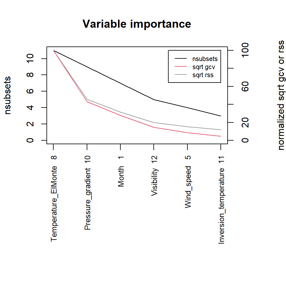
Multivariate Adaptive Regression Splines
The earth package implements variable importance based on multivariate adaptive regression splines (MARS), which is an algorithm that extends linear models to capture nonlinear relationships (Friedman 1991; Friedman 1993). Variable importance is estimated using three criteria: generalized cross validation (GCV), the number of subset models that include the variable (nsubsets), and residual sum of squares (RSS).
library(earth)
marsModel <- earth(ozone_reading ~ ., data = inputData)
ev <- evimp (marsModel)
plot(ev, cex.axis = 0.8, cex.var = 0.8, cex.legend = 0.7)
Stepwise Regression
Stepwise regression consists of iteratively adding and removing predictors, in the predictive model, in order to find the subset of variables in the dataset resulting in the best performing model (Hastie et al. 2016). The step function in base R uses the Akaike information criterion (AIC) for weighing the choices, which takes proper account of the number of parameters fit; at each step an add or drop will be performed that minimizes the AIC score. The AIC rewards models that achieve a high goodness-of-fit score and penalizes them if they become overly complex. By itself, the AIC score is not of much use unless it is compared with the AIC score of a competing model. The model with the lower AIC score is expected to have a superior balance between its ability to fit without overfitting the data (Hastie et al. 2016).
# First fit the base (intercept only) model
base.mod <- lm(ozone_reading ~ 1 , data = inputData)

# Now run stepwise regression with all predictors using a hybrid
# stepwise-selection strategy that considers both forward and
# backward moves at each step, and select the best of the two.
all.mod <- lm(ozone_reading ~ . , data = inputData)
stepMod <- step(
  base.mod, scope = list(lower = base.mod, upper = all.mod),
  direction = "both", trace = 0, steps = 1000
)

# Get the shortlisted variables
shortlistedVars <- names(unlist(stepMod[[1]]))

# Remove intercept
shortlistedVars <- shortlistedVars[!shortlistedVars %in% "(Intercept)"]
data.frame(shortlistedVars = shortlistedVars)
##         shortlistedVars
## 1  Temperature_Sandburg
## 2              Humidity
## 3   Temperature_ElMonte
## 4                 Month
## 5       pressure_height
## 6 Inversion_base_height
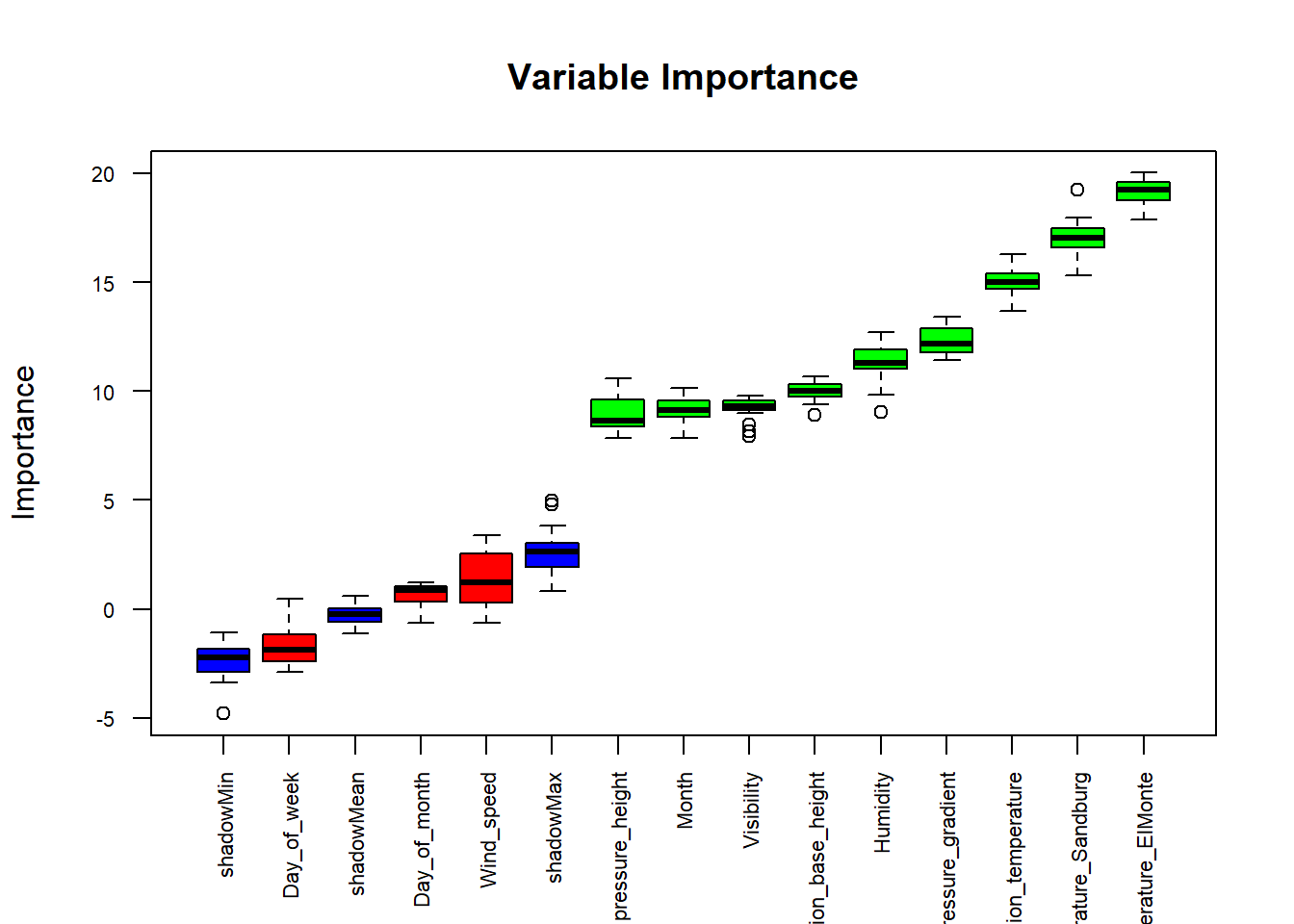
Boruta
The Boruta function is a wrapper algorithm, capable of working with any classification method that outputs variable importance measures (Kursa and Rudnicki 2010). By default, Boruta uses Random Forest. The method performs a top-down search for relevant features by comparing original attribute importance with importance achievable at random, estimated using their permuted copies, and progressively eliminating irrelevant features to stabilise the test.
Boruta follows an all-relevant feature selection method where it captures all features which are in some circumstances relevant to the outcome variable. In contrast, traditional feature selection algorithms follow a minimal optimal method where they rely on a small subset of features which yields a minimal error on a chosen classifier.
library(Boruta)
borout <- Boruta(ozone_reading ~ ., data = na.omit(inputData),
                 doTrace = 2)
boruta_signif <-
  names(borout$finalDecision[borout$finalDecision %in% c("Confirmed", "Tentative")])
data.frame(boruta_signif)
##           boruta_signif
## 1                 Month
## 2       pressure_height
## 3              Humidity
## 4  Temperature_Sandburg
## 5   Temperature_ElMonte
## 6 Inversion_base_height
## 7     Pressure_gradient
## 8 Inversion_temperature
## 9            Visibility
plot(
  borout, cex.axis = 0.7, las = 2,
  xlab = "", main = "Variable Importance"
)
Information Value and Weight of Evidence
The InformationValue package provides convenient functions to compute weights of evidence (WOE) and information value (IV) for categorical variables. The WOE and IV approach evolved from logistic regression techniques. WOE provides a method of recoding a categorical x variable to a continuous variable. For each category of a categorical variable, the WOE is calculated as:
$$WOE = ln\left(\frac{percentage\ good\ of\ all\ goods}{percentage\ bad\ of\ all\ bads}\right)$$
IV is a measure of a categorical x variables ability to accurately predict the goods and bads. For each category of x, the IV is computed as:
$$IV_{category} = \left(\frac{percentage\ good\ of\ all\ goods - percentage\ bad\ of\ all\ bads}{WOE}\right)$$
The total IV of a variable is the sum of the IV’s of its categories.
As an example, let’s use the adult data as imported below. The data has 32,561 observations and 14 features. This dataset is often used with machine learning to predict whether a persons income is higher or lower than $50k per year based on their attributes.
# Load data
library(InformationValue)
inputData <- read.csv("./data/adult.csv", header = TRUE)
str(inputData)
## 'data.frame':	32561 obs. of  14 variables:
##  $ age          : int  39 50 38 53 28 37 49 52 31 42 ...
##  $ workclass    : chr  " State-gov" " Self-emp-not-inc" " Private" " Private" ...
##  $ education    : chr  " Bachelors" " Bachelors" " HS-grad" " 11th" ...
##  $ education.1  : int  13 13 9 7 13 14 5 9 14 13 ...
##  $ maritalstatus: chr  " Never-married" " Married-civ-spouse" " Divorced" " Married-civ-spouse" ...
##  $ occupation   : chr  " Adm-clerical" " Exec-managerial" " Handlers-cleaners" " Handlers-cleaners" ...
##  $ relationship : chr  " Not-in-family" " Husband" " Not-in-family" " Husband" ...
##  $ race         : chr  " White" " White" " White" " Black" ...
##  $ sex          : chr  " Male" " Male" " Male" " Male" ...
##  $ capitalgain  : int  2174 0 0 0 0 0 0 0 14084 5178 ...
##  $ capitalloss  : int  0 0 0 0 0 0 0 0 0 0 ...
##  $ hoursperweek : int  40 13 40 40 40 40 16 45 50 40 ...
##  $ nativecountry: chr  " United-States" " United-States" " United-States" " United-States" ...
##  $ above50k     : int  0 0 0 0 0 0 0 1 1 1 ...
We have a number of predictor variables, out of which a few of them are categorical variables. We will analze the data using the WOE and IV functions in the InformationValue package.
factor_vars <- c (
  "workclass", "education", "maritalstatus",
  "occupation", "relationship", "race",
  "sex", "nativecountry"
)

all_iv <- data.frame(
  VARS = factor_vars,
  IV = numeric(length(factor_vars)),
  STRENGTH = character(length(factor_vars)),
  stringsAsFactors = F
)

for (factor_var in factor_vars) {
  all_iv[all_iv$VARS == factor_var, "IV"] <-
    InformationValue::IV(
      X = inputData[, factor_var],
      Y = inputData$above50k
    )

    all_iv[all_iv$VARS == factor_var, "STRENGTH"] <-
      attr(InformationValue::IV(
        X = inputData[, factor_var],
        Y = inputData$above50k),
        "howgood"
    )
}

# Sort
all_iv[order(-all_iv$IV), ]
##            VARS IV       STRENGTH
## 1     workclass  0 Not Predictive
## 2     education  0 Not Predictive
## 3 maritalstatus  0 Not Predictive
## 4    occupation  0 Not Predictive
## 5  relationship  0 Not Predictive
## 6          race  0 Not Predictive
## 7           sex  0 Not Predictive
## 8 nativecountry  0 Not Predictive
Conclusion
Each of these techniques evaluates each predictor without considering the others. Although these methods are common for sifting through large amounts of data to rank predictors, there are a couple of caveats. First, if two predictors are highly correlated with the response and with each other, then the univariate approach will identify both as important. If the desire is to develop a predictive model, highly correlated predictors can negatively impact some models. Second, the univariate importance approach will fail to identify groups of predictors that together have a strong relationship with the response. For example, two predictors may not be highly correlated with the response; however, their interaction may be. Univariate correlations will not capture this predictive relationship.
References
Boehmke, B. and B.M. Greenwell. Hands-On Machine Learbing with R. CRC Press, Boca Raton.
Chevan, A. and M. Sutherland. 1991. Hierarchical partitioning. The American Statistician, 45, 90-96.
Friedman, J.H. 1991. Multivariate adaptive regression splines. Ann Appl. Stat, 19, 1-141.
Friedman, J.H. 1993. Fast MARS. Stanford University Department of Statistics, Technical Report 110, May.
Guyon, I. and A. Elisseeff. 2003. An introduction to variable and feature selection. Journal of Machine Learning Reserach, 3, 1157-1182.
Hastie, T., R. Tibshirani, and J. Friedman. 2016. The Elements of Statistical Learning: Data Mining, Inference, and Prediction, Second Edition. Springer, New York.
James, G., D. Witten, T. Hastie, and R Tibshirani. An Introudction to Statistical Learning. Springer, New York.
Kuhn, M. and K. Johnson. 2016. Applied Predictive Modeling. Springer, New York.
Kursa, M.B. and W.R. Rudnicki. 2010. Feature selection with the Boruta package. Journal of Statistical Software, 36, 1-13.
Lindeman, R.H., P.F. Merenda, and R.Z. Gold. 1980. Introduction to Bivariate and Multivariate Analysis, Glenview IL: Scott, Foresman.
Reshef, Y.A., D. N. Reshef, H. K. Finucane, P. C. Sabeti, and M. Mitzenmacher. 2016. Measuring Dependence Powerfully and Equitably. Journal of Machine Learning Research, 17, 1-63.
Reshef, D.N., Y. A. Reshef, P. C. Sabeti, and M. Mitzenmacher. 2018. An empirical study of the maximal and total information coefficients and leading measures of dependence. Ann Appl. Stat, 12, 123-155.
- Posted on:
- February 14, 2020
- Length:
- 17 minute read, 3586 words
- See Also: