Fitting Distributions with Censored Data
By Charles Holbert
June 26, 2019
Introduction
The term “distribution” is used frequently in statistics. Many statistical analyses depend on the type of data distribution. This includes computation of basic descriptive statistics, probabilistic statements about the data population based on sample statistics (e.g., the proportion or percentage of the data population that is higher or lower than a specified value), tests of hypothesis, regression analysis, and so on. Parametric testing methods assume that the type of underlying distribution is at least approximately known or can be identified through diagnostic testing. When analyzing small data sets, distributional assumptions are important for estimating upper threshold values, such as the 90th or 95th percentile, or a 95 percent upper confidence limit (UCL95) on the mean value. For larger sample sizes (20 or more observations), other methods are available that don’t rely on an assumed distribution.
A large variety of possible distributional models exist in the statistical literature. Statistical models for the environmental sciences are usually confined to the lognormal distribution, the gamma distribution, the Weibull distribution, or distributions that are normal or can be normalized via a transformation (e.g., the logarithmic or square root). Tests that determine whether a distribution fits the data are known as goodness-of-fit (GOF) tests. GOF tests are used to test the null hypothesis that the data come from a particular family of distributions, such as “the data come from a lognormal distribution.” Probability plots (also known as quantile-quantile [Q-Q] plots) also are used for assessing data distribution.
Q-Q Plots
Q-Q plots are used to check the similarity of data to a specified distribution. However, standard Q-Q plots are not designed for censored (containing non-detects) data. As an example, let’s consider arsenic concentrations in groundwater containing four censoring limits: 0.5, 2, 3, and 4 micrograms per liter. Reported concentrations are listed in the As variable and detect/non-detect qualifiers (TRUE for non-detects and FALSE for detects) are provided in the Ascen variable.
# Load libraries
library(NADA)
library(fitdistrplus)
library(EnvStats)

# Create censored data set
As <- c(
  0.5, 2, 3, 4, 4,
  4, 4, 4, 4, 4,
  4, 4, 4, 4, 1.2,
  0.6, 0.53, 3.8, 4.1, 4.85,
  5.27
)

Ascen <- c(
  TRUE, TRUE, TRUE, TRUE, TRUE,
  TRUE, TRUE, TRUE, TRUE, TRUE,
  TRUE, TRUE, TRUE, TRUE, FALSE,
  FALSE, FALSE, FALSE, FALSE, FALSE,
  FALSE
)
Let’s create a data frame that includes columns left and right, describing each observed value as an interval. The left column contains either NA for non-detects or the observed value for detected observations. The right column contains either the detection limit for non-detects or the observed value for detected observations. This format is required for using the R package tdistrplus (Delignette-Muller, 2018).
# Create dataframe with left/right columns for fitdistrplus
dat <- data.frame(As, Ascen)
dat$Ashalf <- ifelse(dat$Ascen == TRUE, 0.5 * dat$As, dat$As)
dat$left <- ifelse(dat$Ascen == TRUE, NA, dat$As)
dat$right <- As
Let’s inspect the data.
# Generate summary of data
censummary(As, Ascen)
## all:
##        n    n.cen  pct.cen      min      max
## 21.00000 14.00000 66.66667  0.50000  5.27000
##
## limits:
##   limit  n uncen   pexceed
## 1   0.5  1     3 0.8163265
## 2   2.0  1     0 0.2653061
## 3   3.0  1     1 0.2653061
## 4   4.0 11     3 0.1428571
Now, let’s create Q-Q plots for the following scenarios: (1) non-detects equal to one-half the detection limit; (2) non-detects equal to the detection limit; and (3) non-detects ignored (detects only). Let’s also create a censored Q-Q plot where plotting positions properly account for the presence of non-detects.
# Create qqplots for normal distribution

# Create qqplot for:

# 1. non-detects equal to one-half censoring limit
# 2. non-detects equal to censoring limit
# 3. detects only

par(mfrow = c(2, 2))
qqPlot(
  dat$Ashalf, dist = "norm",
  add.line = TRUE, pch = 16, cex = 1.2,
  ylab = "As Concentration",
  main = "Arsenic, nondetects equal one-half DL"
)

qqPlot(
  As, dist = "norm",
  add.line = TRUE, pch = 16, cex = 1.2,
  ylab = "As Concentration",
  main = "Arsenic, nondetects equal DL"
)

qqPlot(
  dat[Ascen == FALSE,]$As, dist = "norm",
  add.line = TRUE,  pch = 16, cex = 1.2,
  ylab = "As Concentration",
  main = "Arsenic, detects only"
)

qqPlotCensored(
  As, Ascen, dist = "norm",
  add.line = TRUE,  pch = 16, cex = 1.2,
  ylab = "As Concentration"
)
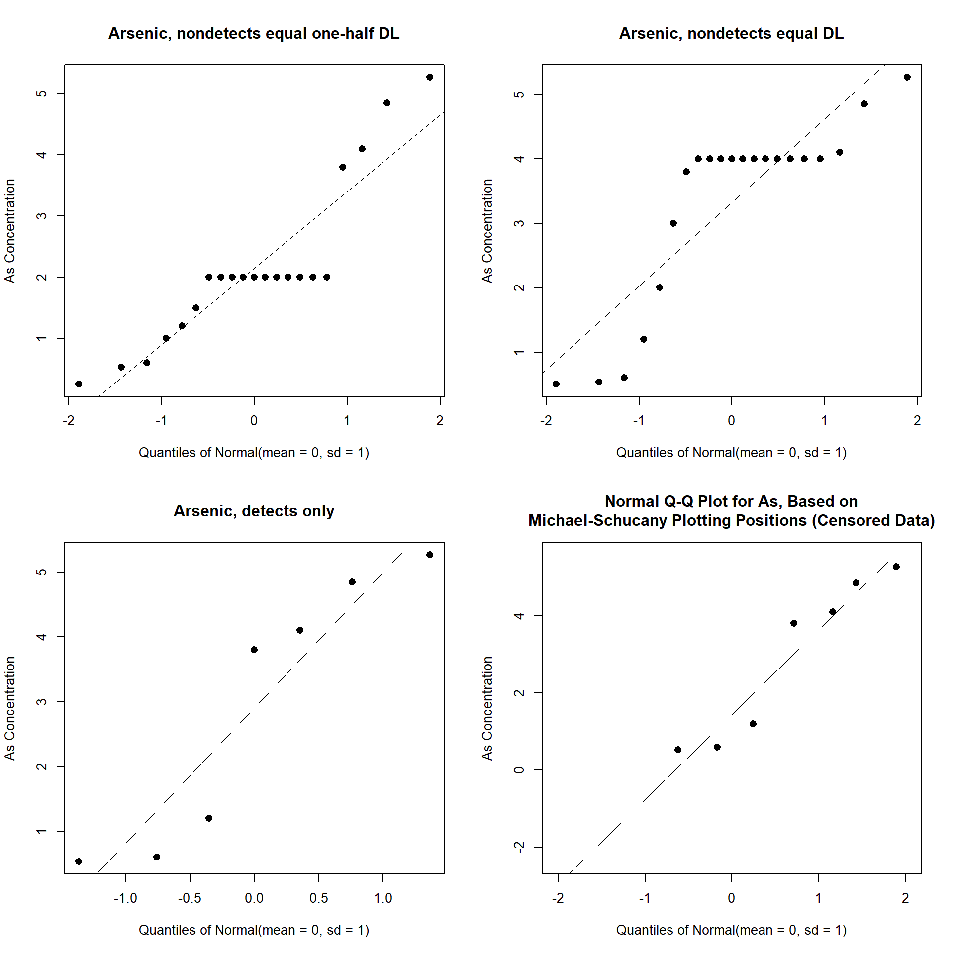
When non-detects are assumed equal to the detection limit or some fraction of the detection limit, the substituted values form straight lines in the Q-Q plot. When non-detects are simply ignored, the percentiles are too low (pushed to the left). In all these situations, the distribution at the low end is distorted compared to the true shape of the data. Typically, this leads to choosing the wrong distribution and incorrect statistical estimates. In the censored Q-Q plot, non-detects are not plotted but appropriate space is left for them so that percentiles for the detected observations are correct. The correct plotting positions are determined using techniques from survival analysis (Millard 2013).
Fitting Distributions
Now, let’s fit three distributions (normal, lognormal, and gamma) to the censored data using maximum likelihood estimation (MLE). In MLE, optimization is performed to maximize the match between the observed data and the estimated distribution parameters. For censored data, the computed percentiles incorporate both the detected observations and the proportions of data (detects and non-detects) below each detection limit (Helsel 2012).
# Fit distributions using MLE in fitdistrplus
fits.norm <- fitdistcens(dat[, 4:5], "norm")
fits.lnorm <- fitdistcens(dat[, 4:5], "lnorm")
fits.gamma <- fitdistcens(dat[, 4:5], "gamma")

# Create graphical comparison of fitted distributions using fitdistrplus
cdfcompcens(list(fits.gamma, fits.lnorm, fits.norm), xlim = c(-2, 6))
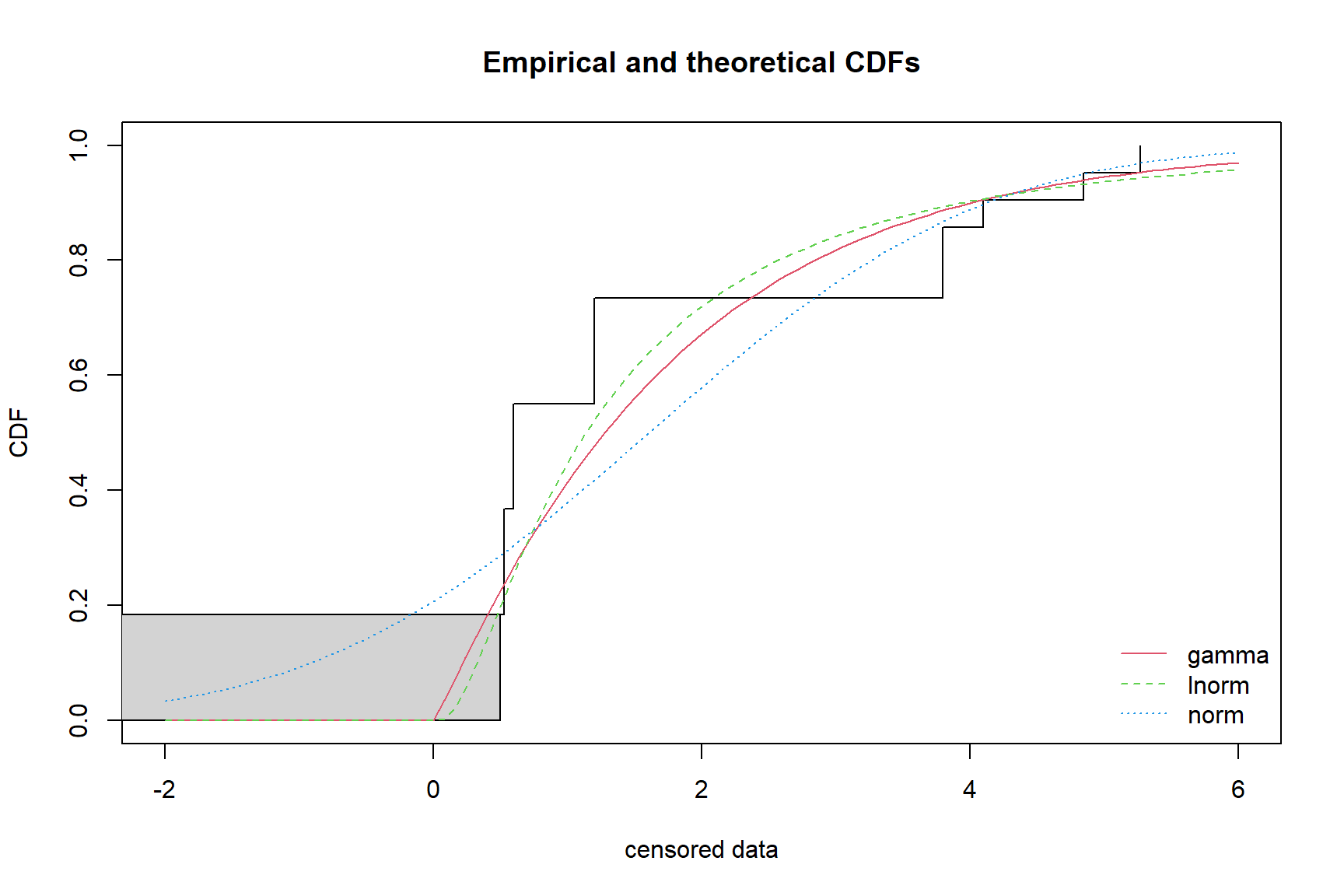
In the plot of the empirical cumulative distribution against the fitted distribution functions, the observed data are shown as a step function. For our case, the gamma and lognormal distributions appear to provide the best fit to the data. Note that the normal distribution estimates concentrations below zero. In practice, many environmental data sets follow a lognormal as well as a gamma distribution. Because a lognormal distribution on a lognormally distributed data set may yield impractically large upper threshold values, a gamma distribution typically is given preference over a lognormal distribution (USEPA 2015).
Let’s perform a GOF tests for a gamma distribution using the censored data.
# Goodness-of-fit test for gamma distribution
gamma_gof <- gofTestCensored(As, Ascen, dist = "gamma", test = "ppcc")
print(gamma_gof)
##
## Results of Goodness-of-Fit Test
## Based on Type I Censored Data
## -------------------------------
##
## Test Method:                     PPCC GOF
##                                  (Multiply Censored Data)
##                                  Based on Chen & Balakrisnan (1995)
##
## Hypothesized Distribution:       Gamma
##
## Censoring Side:                  left
##
## Censoring Level(s):              0.5 2.0 3.0 4.0
##
## Estimated Parameter(s):          shape = 1.091381
##                                  scale = 1.630625
##
## Estimation Method:               MLE
##
## Data:                            As
##
## Censoring Variable:              Ascen
##
## Sample Size:                     21
##
## Percent Censored:                66.66667%
##
## Test Statistic:                  r = 0.9609473
##
## Test Statistic Parameters:       N     = 21.0000000
##                                  DELTA =  0.6666667
##
## P-value:                         0.5620572
##
## Alternative Hypothesis:          True cdf does not equal the
##                                  Gamma Distribution.
Let’s perform a GOF tests for a lognormal distribution using the censored data.
# Goodness-of-fit test for lognormal distribution
lnorm_gof <- gofTestCensored(As, Ascen, dist = "lnorm", test = "ppcc")
print(lnorm_gof)
##
## Results of Goodness-of-Fit Test
## Based on Type I Censored Data
## -------------------------------
##
## Test Method:                     PPCC GOF
##                                  (Multiply Censored Data)
##
## Hypothesized Distribution:       Lognormal
##
## Censoring Side:                  left
##
## Censoring Level(s):              0.5 2.0 3.0 4.0
##
## Estimated Parameter(s):          meanlog = 0.1280339
##                                  sdlog   = 0.9700502
##
## Estimation Method:               MLE
##
## Data:                            As
##
## Censoring Variable:              Ascen
##
## Sample Size:                     21
##
## Percent Censored:                66.66667%
##
## Test Statistic:                  r = 0.9551052
##
## Test Statistic Parameters:       N     = 21.0000000
##                                  DELTA =  0.6666667
##
## P-value:                         0.4609222
##
## Alternative Hypothesis:          True cdf does not equal the
##                                  Lognormal Distribution.
Let’s perform a GOF tests for a normal distribution using the censored data.
# Goodness-of-fit test for normal distribution
norm_gof <- gofTestCensored(As, Ascen, dist = "norm", test = "ppcc")
print(norm_gof)
##
## Results of Goodness-of-Fit Test
## Based on Type I Censored Data
## -------------------------------
##
## Test Method:                     PPCC GOF
##                                  (Multiply Censored Data)
##
## Hypothesized Distribution:       Normal
##
## Censoring Side:                  left
##
## Censoring Level(s):              0.5 2.0 3.0 4.0
##
## Estimated Parameter(s):          mean = 1.605237
##                                  sd   = 1.969153
##
## Estimation Method:               MLE
##
## Data:                            As
##
## Censoring Variable:              Ascen
##
## Sample Size:                     21
##
## Percent Censored:                66.66667%
##
## Test Statistic:                  r = 0.9649854
##
## Test Statistic Parameters:       N     = 21.0000000
##                                  DELTA =  0.6666667
##
## P-value:                         0.6390037
##
## Alternative Hypothesis:          True cdf does not equal the
##                                  Normal Distribution.
The highest Probability Plot Correlation Coefficient (PPCC) test statistic is for the normal distribution (PPCC of 0.965), although it’s almost the same as that for the gamma distribution (PPCC of 0.961). Recall, that the fitted normal distribution predicted negative concentrations as shown in the censored Q-Q plot and the plot of the cumulative distribution function. Because of this, the normal distribution would not be ideally suited for statistical estimation purposes.
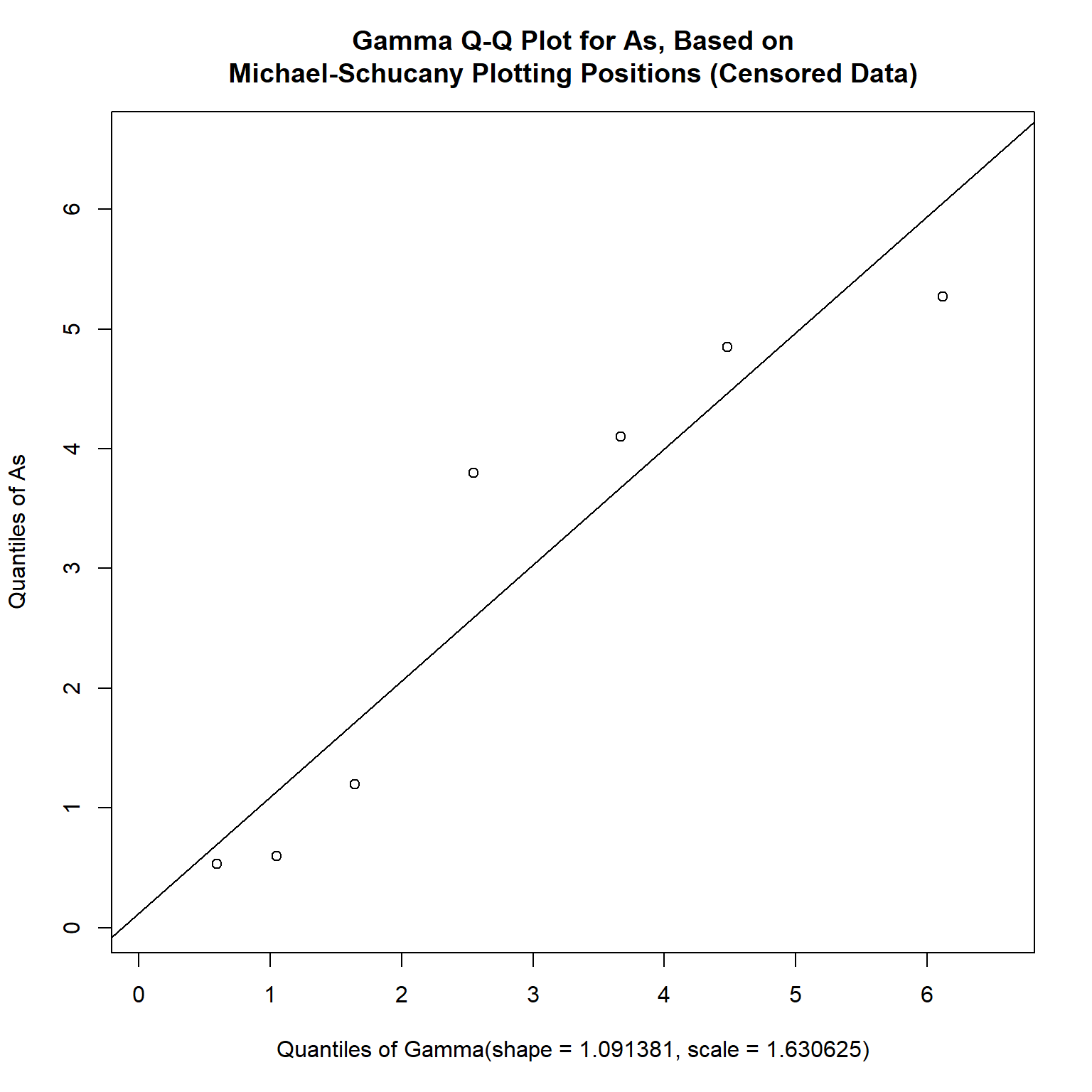
Selecting the gamma distribution as the best fit to our data, a censored Q-Q plot can be created as follows:
# Create censored qqplot for gamma distribution using EnvStats
qqPlotCensored(
  As, Ascen, dist = "gamma",
  add.line = TRUE,
  estimate.params = T
)
Now that we have fitted a distribution to our data, we can calculate the mean, coefficient of variation, and the UCL95.
# Compute mean and UCL95 using EnvStats
sum_stats <- egammaAltCensored(
  As, Ascen,
  ci = TRUE, ci.type = "upper",
  ci.method = "normal.approx"
)
print(sum_stats)
##
## Results of Distribution Parameter Estimation
## Based on Type I Censored Data
## --------------------------------------------
##
## Assumed Distribution:            Gamma
##
## Censoring Side:                  left
##
## Censoring Level(s):              0.5 2.0 3.0 4.0
##
## Estimated Parameter(s):          mean = 1.7796323
##                                  cv   = 0.9572201
##
## Estimation Method:               MLE
##
## Data:                            As
##
## Censoring Variable:              Ascen
##
## Sample Size:                     21
##
## Percent Censored:                66.66667%
##
## Confidence Interval for:         mean
##
## Confidence Interval Method:      Normal Approximation
##
## Confidence Interval Type:        upper
##
## Confidence Level:                95%
##
## Confidence Interval:             LCL =     -Inf
##                                  UCL = 2.519906
Because we selected an upper confidence limit, the lower confidence limit (LCL) is listed as -Inf. We also can calculate the 90th and 95th percentiles as follows:
# Compute upper percentiles using EnvStats
As.gamma <- egammaCensored(As, Ascen)
perc <- eqgamma(As.gamma, p = c(0.90, 0.95))
print(perc)
##
## Results of Distribution Parameter Estimation
## Based on Type I Censored Data
## --------------------------------------------
##
## Assumed Distribution:            Gamma
##
## Censoring Side:                  left
##
## Censoring Level(s):              0.5 2.0 3.0 4.0
##
## Estimated Parameter(s):          shape = 1.091381
##                                  scale = 1.630625
##
## Estimation Method:               MLE
##
## Estimated Quantile(s):           90'th %ile = 4.010268
##                                  95'th %ile = 5.169756
##
## Quantile Estimation Method:      Quantile(s) Based on
##                                  MLE Estimators
##
## Data:                            As
##
## Censoring Variable:              Ascen
##
## Sample Size:                     21
##
## Percent Censored:                66.66667%
References
Delignette-Muller, M. L. 2018. fitdistrplus: An R Package for Fitting Distributions. July.
Helsel, D. R. 2012. Statistics for Censored Environmental Data using Minitab and R, 2nd edition. New York: John Wiley & Sons.
Millard, S.P. 2013. EnvStats: An R Package for Environmental Statistics. Springer, NY.
U.S. Environmental Protection Agency (USEPA). 2015. ProUCL Version 5.1 Technical Guide. EPA/600/R-07/041. October.
- Posted on:
- June 26, 2019
- Length:
- 9 minute read, 1904 words
- See Also: