Introduction

Costs for groundwater monitoring represent a significant, persistent, and growing burden for private entities and government agencies responsible for environmental remediation projects. With the increasing use of risk-based goals and natural attenuation, the need for better-designed long-term groundwater monitoring (LTM) well networks that are both cost-effective and protective of human and environmental health has greatly increased. Many existing LTM networks, either developed during site characterization activities or in the initial stages of groundwater remediation, do not reflect changes in site conditions, resulting in too many wells being sampled too often.

Groundwater monitoring well networks have to be designed, evaluated, and sometimes enlarged or reduced. Optimization of LTM networks offers an opportunity to improve the cost-effectiveness of monitoring by ensuring objectives are achieved with an appropriate level of effort. Optimization may identify redundancies in the monitoring program that can be removed or inadequacies that may require changes in the monitoring program to protect against potential impacts to the environment. The difficulty of finding optimal well network designs is that a quantitative criterion is often a priori not present.

This factsheet is the first of three factsheets that uses geostatistical methods to spatially optimize groundwater monitoring well networks. For this first factsheet, a simple approach is used to identify where new wells should be located or which well locations should be removed such that the operational value of the monitoring network is maximized. The second factsheet will describe the use of Sequential Gaussian Simulation (SGSIM) conditioned on measured groundwater concentration data to assess spatial variability in the predicted distribution of contamination. The third and last factsheet will conduct geospatial optimization of a groundwater monitoring well network with the objective of minimizing the number of sample locations needed to represent the plume, subject to the constraint that the characteristics of the plume remain comparable.

Methodology

Geostatistical data are data that could in principle be measured anywhere, but that typically come as measurements at a limited number of observation locations. The interest in collecting these data is usually in inference of aspects of the variable that have not been measured, such as maps of the estimated values, exceedence probabilities, or estimates of aggregates over given regions. Geostatistical techniques based on semivariogram modeling and kriging are generally used to eliminate spatially redundant sampling locations. Spatial redundancy is caused by monitoring wells that contribute little additional information regarding plume characterization because of their spatial correlation with other monitoring wells.

Kriging

Kriging, developed by the South African mining engineer D. G. Krige (1951) and latter formalized by the French geologist and statistician Georges Matheron (1963), is a family of estimators used to interpolate spatial data. Kriging is an interpolation technique that calculates a concentration at an unknown location through a weighted average of known points within a data-specific neighborhood. Kriging is a global estimator in that its estimate represents all data within a defined area. In general, kriging weights are calculated such that points nearby to the location of interest are given more weight than those farther away. Each interpolated value is calculated to minimize the prediction error for that point. Ordinary kriging (Isaaks and Srivastava 1989; Gooevaerts 1997) is one of the simplest forms of kriging. It assumes a constant but unknown mean over the search neighborhood.

If there is little spatial autocorrelation among the sampled data points, kriging will not be more effective than simpler methods of interpolation. However, kriging helps preserve the spatial variability that would be lost using a simpler method for those data with at least a moderate level of spatial autocorrelation. The accuracy of interpolation by kriging will be limited if the number of sampled observations is small, the data are limited in spatial scope, or the data are not spatially correlated. In these cases, a sample variogram is difficult to generate.

Well Network Optimization Methodology

A simple approach for monitoring well network optimization is to express the doubt about whether a location is below or above a specified isoconcentration contour level. For example, to delineate the 5 micrograms per liter (µg/L) contour, we can express the doubt about whether a location is below or above 5 µg/L as the closeness of \(G((\hat{Z}(s_0) - 5)/\sigma(s_0))\) to 0.5, where \(G(\cdot)\) is the Gaussian distribution function and \(\sigma\) is the standard deviation. For adding wells, the Gaussian distribution function is looped over a fixed grid to identify the location that increases the objective function most. Identifying locations for adding wells is computationally more intensive as the number of options for addition are much larger than those for removal.

Parameters

Several libraries, functions, and parameters are required to perform the spatial optimization.

# Load libraries
library(dplyr)
library(rgdal)
library(raster)
library(geoR)
library(gstat)

# Load functions
source('functions/SumStats.R')

# Set options so no scientific notation
options(scipen = 999)

# Set parameters
expand <- 'Y'         # Expand interpolation grid outside data domain ('Y' or 'N')
nodes <- 400          # Number of grid nodes
epsg <- 2229          # European Petroleum Survey Group (EPSG) code
threshold <- 5        # threshold for plotting
options(scipen = 999) # Disable scientific notation

# Create color-scale for plots
leg <- c(
  "#0000ff", "#0028d7", "#0050af", "#007986", "#00a15e",
  "#00ca35", "#00f20d", "#1aff00", "#43ff00", "#6bff00",
  "#94ff00", "#bcff00", "#e5ff00", "#fff200", "#ffca00",
  "#ffa100", "#ff7900", "#ff5000", "#ff2800", "#ff0000"
)

# Create breaks for legend
axis.ls <- list(
  at = c(log10(5), 1, 2, 3, 4),
  labels = c(5, 10, 100, 1000, 10000)
)

# Funtion for suppressing output
quiet <- function(x) { 
  sink(tempfile()) 
  on.exit(sink()) 
  invisible(force(x)) 
}

Data

The data used in this example consist of benzene concentrations measured during a single sampling event. Results are given in µg/L. The data consist of a mixture of detects and non-detects. The non-detects have been assigned a value of 0.1 µg/L. The groundwater monitoring well network corresponding to the benzene concentration data consists of 25 groundwater monitoring wells installed in an unconfined perched groundwater system, located within an alluvial deposit.

Summary Statistics

The structure of the data is shown below and consists of eight variables. The variables include well id, parameter name, measurement result, units of measure, whether the result is a detect (“Y”) or non-detect (“N”), the water-bearing zone where the well is installed, and geographical coordinates for each well given in feet.

# Load data
datin <- read.csv('data/benzene.csv', header = T)

# View structure of data
str(datin)

## 'data.frame':	25 obs. of  8 variables:
##  $ LOCID : chr  "CP-1" "MW-01A" "MW-05" "MW-06" ...
##  $ PARAM : chr  "Benzene" "Benzene" "Benzene" "Benzene" ...
##  $ RESULT: num  0.1 0.1 330 93 4.8 0.1 0.1 1100 320 20 ...
##  $ UNITS : chr  "ug/L" "ug/L" "ug/L" "ug/L" ...
##  $ DETECT: chr  "N" "N" "Y" "Y" ...
##  $ ZONE  : chr  "P" "P" "P" "P" ...
##  $ XCOORD: num  6456449 6456526 6456397 6456256 6456274 ...
##  $ YCOORD: num  1769548 1769232 1769286 1769363 1769183 ...

Summary statistics of the benzene concentrations are shown below. There are 25 results with 16 detects, corresponding to a detection frequency of 64 percent. The minimum and maximum concentrations are <1 and 2,500 µg/L, respectively. The mean concentration is 235.6 µg/L with a median concentration of 4.1 µg/L and a standard deviation of 541.9 µg/L. The coefficient of variation (CV) is 2.3, indicating a highly skewed data set. The Kaplan-Meier (KM) product-limit estimator (Kaplan and Meier 1958) was used to compute the summary statistics.

# Get summary statistics and transpose
zz <- SumStats(datin, rv = 1)
names <-  zz[,1]  # keep 1st column
zz.T <- data.frame(as.matrix(t(zz[,-1])))  # transpose everything but 1st column
colnames(zz.T) <- names  # assign 1st column as column names
zz.T

##         Benzene
## Obs        25.0
## Dets       16.0
## DetFreq    64.0
## MinND       0.1
## MinDET      1.8
## MaxND       0.1
## MaxDet   2500.0
## Mean      235.6
## Median      4.1
## SD        541.9
## CV          2.3

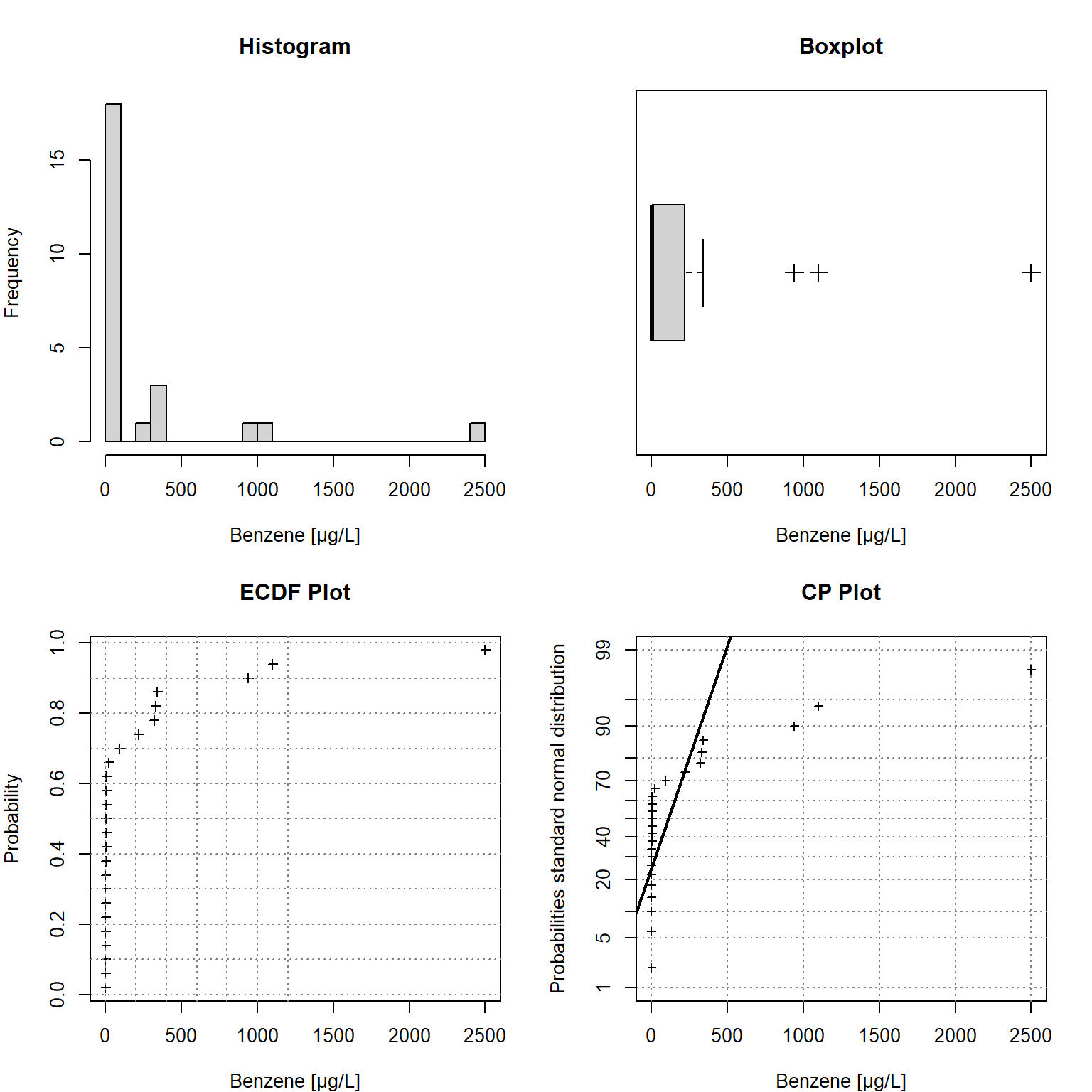
Univariate Statistical Graphics

Univariate statistical plots are provided below. These plots can be used to understand the characteristics of the observed data, including the data distribution; the median, skewness, and tailedness of the distribution; and to identify data outliers. The plots include a histogram in the upper left window, an empirical cumulative density function (ECDF) plot in the lower left window, a box plot in the upper right window, and a cumulative probability (CP) plot in the lower right window. As shown in the plots, the data are strongly right-skewed. The comparison with probabilities of the (standard) normal distribution in the CP plot indicates the data are not normally distributed.

# Load data
Benzene <- datin[,"RESULT"]
n <- length(Benzene)

# Set plotting window for 2 x 2 plots
par(mfcol = c(2, 2), mar = c(4, 4, 4, 2))

# Plot 1. Histogram
hist(
  Benzene,
  breaks = 25,
  main = "",
  xlab = "Benzene [µg/L]",
  ylab = "Frequency",
  cex.lab = 1
)
title("Histogram")

# Plot 2. Empirical Cumulative Density Function Plot
plot(
  sort(Benzene),
  ((1:n) - 0.5)/n,
  pch = 3, cex = 0.8,
  main = "",
  xlab = "Benzene [µg/L]",
  ylab = "Probability",
  cex.lab = 1
)
abline(h = seq(0, 1, by = 0.1), lty = 3, col = gray(0.5))
abline(v = seq(0, 1200, by = 200), lty = 3,col = gray(0.5))
title("ECDF Plot")

# Plot 3. Boxplot
boxplot(
  Benzene,
  horizontal = T,
  xlab = "Benzene [µg/L]",
  cex.lab = 1, pch = 3, cex = 1.5
)
title("Boxplot")

# Plot 4. Quantile-Probability Plot
StatDA::qpplot.das(
  Benzene,
  qdist = qnorm,
  xlab = "Benzene [µg/L]",
  ylab = "Probabilities standard normal distribution",
  pch = 3, cex = 0.7, cex.lab = 1,
  logx = FALSE
)
title("CP Plot")

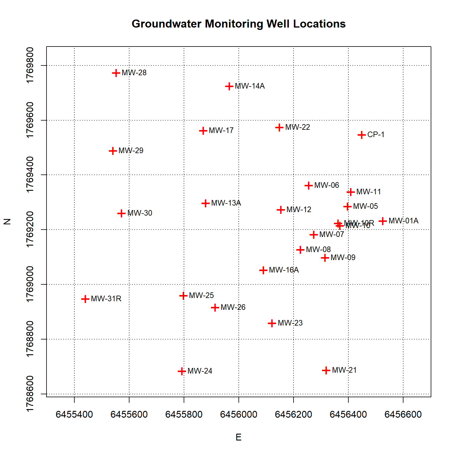
Spatial Data Structure

A plot of each groundwater monitoring well location along with its label is shown below. The locations are relatively well-distributed across the site with some localized clustering in the central portion of the site near the eastern boundary.

# Prep data
dat <- datin %>%
  dplyr::select(XCOORD, YCOORD, RESULT, LOCID) %>%
  dplyr::rename(
    x = XCOORD,
    y = YCOORD,
    conc = RESULT,
    locid = LOCID
  )

# Make data geospatial object
coordinates(dat) = ~x+y
proj4string(dat) = CRS(paste0("+init=epsg:", epsg))

# Plot the locations of each station along with its label
plot(
  coordinates(dat),
  xlim = c(6455350, 6456650),
  pch = "+", col = "red", cex = 1.8,
  asp = 1,
  xlab = "E", ylab = "N",
  main = "Groundwater Monitoring Well Locations"
)
grid(lwd = 1.4, col = "grey20")
text(coordinates(dat), labels = dat@data$locid, pos = 4, cex = 0.8)

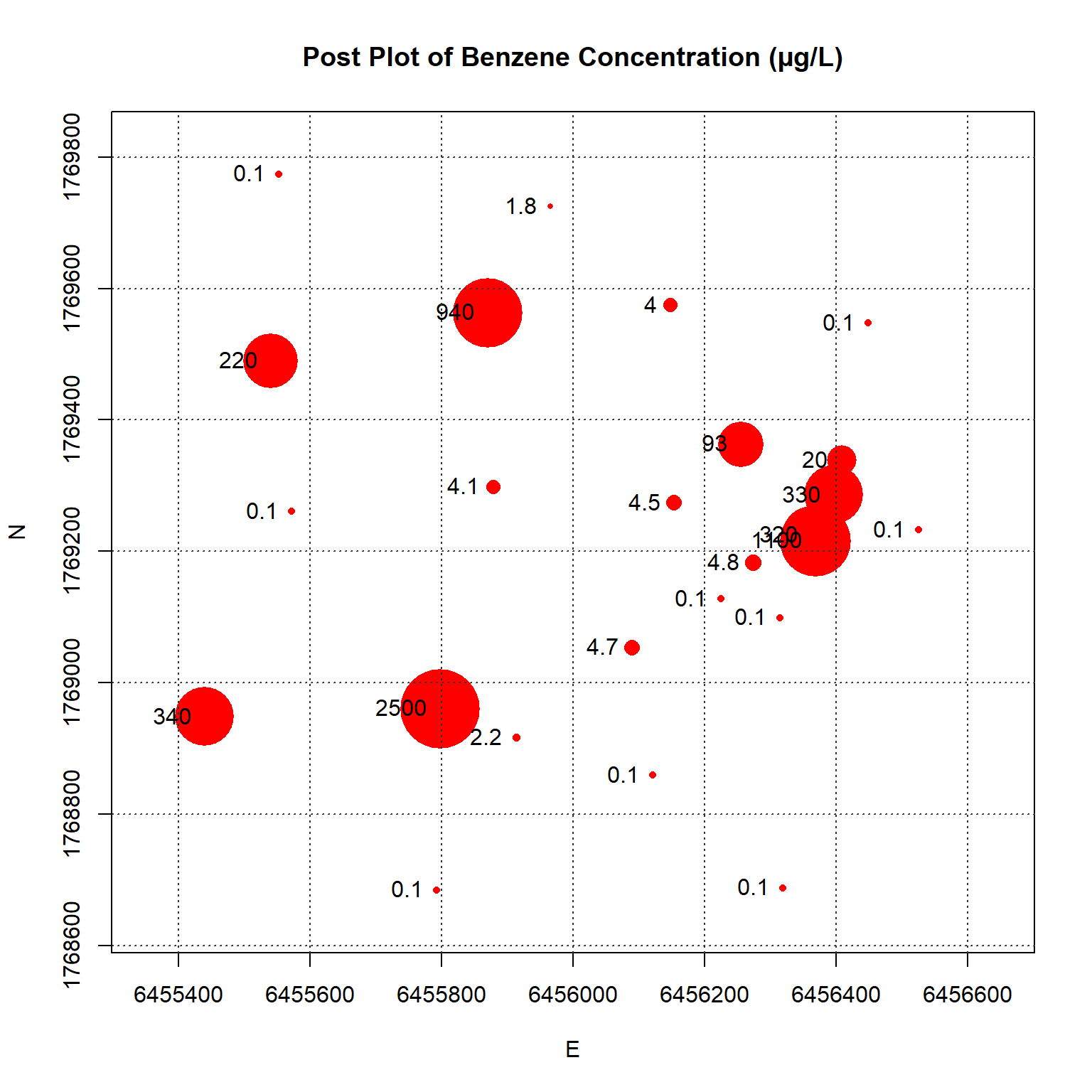
A post-plot of the benzene concentration at each monitoring well is shown below. The size of each symbol reflects the actual concentration at that location; larger symbols equate to higher concentrations on a log scale. The plot indicates higher benzene concentrations located within the interior of the monitoring well network with lower concentrations along the outer hull of the network.

# Make a post-plot of concentrations
plot(
  coordinates(dat),
  xlim = c(6455350, 6456650),
  pch = 16, col = "red", asp = 1,
  cex = ifelse(dat@data$conc == 0.1, log(20*dat@data$conc), log(dat@data$conc)),
  #cex = 10*dat@data$conc/max(na.omit(dat@data$conc)),
  xlab = "E", ylab = "N",
  main = "Post Plot of Benzene Concentration (µg/L)"
)
text(coordinates(dat), labels = round(dat@data$conc, 2), pos = 2)
grid(lwd = 1.4, col = "grey20")

Well Network Optimization

Ordinary kriging was used to interpolate benzene concentrations in groundwater at the site. An omnidirectional variogram was fit to the log-transformed data using an exponential model with a range of 1,000 feet and a sill of 4. Lognormal transformation was used to change the shape of the frequency distribution of the highly skewed distribution of the data. This normalization step reduces data variance and improves the calculation of statistics and weighted averages, such as ordinary kriging estimates. Kriging was conducted using a rectilinear grid 2,390 feet wide (Easting direction) and 1,520 feet long (Northing direction). The grid spacing was 5.975 feet in the x-direction and 3.8 feet in the y-direction. The model domain contained a total of 160,000 nodes.

# Setup grid using data extents
delx <- (max(dat@coords[,1]) - min(dat@coords[,1]))*0.6
dely <- (max(dat@coords[,2]) - min(dat@coords[,2]))*0.2

if (expand == 'Y') {
  xb <- round(min(dat@coords[,1]) - delx, -1)
  xe <- round(max(dat@coords[,1]) + delx, -1)
  yb <- round(min(dat@coords[,2]) - dely, -1)
  ye <- round(max(dat@coords[,2]) + dely, -1)
} else {
  xb <- min(dat@coords[,1])
  xe <- max(dat@coords[,1])
  yb <- min(dat@coords[,2])
  ye <- max(dat@coords[,2])
}

xn <- (xe - xb)/nodes
yn <- (ye - yb)/nodes
grid2D <- expand.grid(
  x = seq(xb, xe, xn),
  y = seq(yb, ye, yn)
)
gridded(grid2D) <- ~x+y
proj4string(grid2D) = CRS(paste0("+init=epsg:", epsg))

# Convert from SpatialPixels to SpatialPixelsDataFrame
grid2D.spdf <- SpatialPixelsDataFrame(
  grid2D,
  data = data.frame(grid2D)
)

# Create variogram using omnidirectional variogram
v <- variogram(log10(conc) ~ 1, dat)
v.fit <- fit.variogram(v, vgm(6, "Exp", 1000))
v.fit$psill <- 4
v.fit$range <- 1000

# Kriging
conc.gstat <- quiet(
  krige(log10(conc) ~ 1, dat, grid2D, model = v.fit)
)
pred <- conc.gstat$var1.pred

# Add predictions to spatial pixels object
grid2D.spdf$conc_gstat <- ifelse(pred < log10(5), NA, 10^pred)

The previously defined Gaussian distribution function was used to identify the 10 percent most influential and least influential monitoring wells for delineating the plume based on the 5 µg/L isoconcentration contour. For adding wells, a fixed grid was used to find the point that increased the Gaussian distribution function most. Because identifying locations for well addition is computationally intensive, a coarse grid was defined with a spacing of 119.5 feet in the x-direction, 76 feet in the y-direction, and containing a total of 400 nodes.

# Get most important wells for delineating cutoff threshold value
n <- length(dat@data$conc)
cutoff <- 5
f <- function(x) {
  kr = quiet(krige(log10(conc) ~ 1, dat[-x, ], grid2D, v.fit))
  mean(abs(pnorm((kr$var1.pred - log10(cutoff))/sqrt(kr$var1.var)) - 0.5))
}
m1 <- sapply(1:n, f)
#p <- which(m1 == max(m1))
#dat@data[p, ]

# Setup coarse grid using data extents
xn <- (xe - xb)/20
yn <- (ye - yb)/20
gridNew <- expand.grid(
  x = seq(xb, xe, xn),
  y = seq(yb, ye, yn)
)
gridded(gridNew) <- ~x+y
proj4string(gridNew) = CRS(paste0("+init=epsg:", epsg))

# Get most important locations for adding wells using cutoff value
n <- length(gridNew)
cutoff <- 5
f <- function(x) {
  kr = quiet(krige(log10(conc) ~ 1, dat, gridNew[-x, ], v.fit))
  mean(abs(pnorm((kr$var1.pred - log10(cutoff))/sqrt(kr$var1.var)) - 0.5))
}
m2 <- sapply(1:n, f)

# Rerun using a different cutoff value
cutoff <- 10
m3 <- sapply(1:n, f)

# Rerun using a different cutoff value
cutoff <- 100
m4 <- sapply(1:n, f)

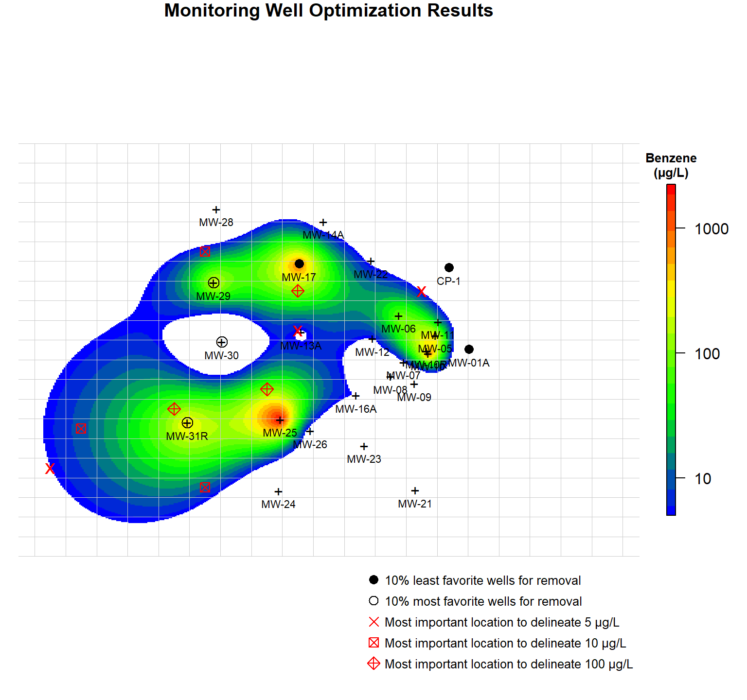
A plot showing benzene contours and candidate points for removal and addition is shown below. Also shown in the plot is the coarse grid that was used to identify possible locations for monitoring well addition. The most favorite and least favorite monitoring wells for removal are shown as open black circles and closed black circles, respectively. Red crosses, red boxes, and red diamonds represent the most favorable locations for adding a well to delineate the 5 µg/L contour, 10 µg/L contour, and 100 µg/L contour, respectively.

# Create plot showing candidate points for removal and addition.
# Open circles ---> 10% most favorite points for removal
# Closed circles ---> 10% least favorite points for removal
# Red crosses ---> most favorite points for addition to delineate 5 ug/L contour
# Red boxes ---> most favorite points for addition to delineate 10 ug/L contour
# Red diamonds ---> most favorite points for addition to delineate 100 ug/L contour

par(mar = c(1, 1, 1, 2))  # bottom, left, top, right; default is c(5.1, 4.1, 4.1, 2.1)
plot(
  log10(raster(grid2D.spdf['conc_gstat'])),
  col = leg,
  main = "Monitoring Well Optimization Results",
  axes = FALSE,
  box = FALSE,
  axis.args = axis.ls,
  legend.args = list(text = "Benzene\n(µg/L)", side = 3, font = 2, line = 0.2, cex = 0.8)
)
plot(gridNew, lwd = 0.05, col = "grey80", add = T)
points(dat, pch = "+")
points(dat[m1 < quantile(m1, 0.1),], pch = 16, cex = 1.3, col = "black")
points(dat[m1 > quantile(m1, 0.9),], pch = 1, cex = 1.6, col = "black")
points(gridNew[m2 > quantile(m2, 0.995),], pch = "x", cex = 1.3, col = "red")
points(gridNew[m3 > quantile(m3, 0.995),], pch = 7, cex = 1.3, col = "red")
points(gridNew[m4 > quantile(m4, 0.995),], pch = 9, cex = 1.3, col = "red")
text(dat, dat@data$locid, cex = 0.7, pos = 1, col = "black")

# Add legend
legend(
  "bottomright",
  legend = c(
    "10% least favorite wells for removal",
    "10% most favorite wells for removal",
    "Most important location to delineate 5 µg/L",
    "Most important location to delineate 10 µg/L",
    "Most important location to delineate 100 µg/L"
  ),
  col = c("black", "black", rep("red", 3)),
  pch = c(16, 1, 4, 7, 9),
  text.font = 1, bty = "n",
  pt.cex = 1.3, cex = 0.8, y.intersp = 1.4
)

When two or more points have to be added or removed jointly, the problem becomes computationally very intensive, as the sequential solution (first the best point, then the second best) is not necessarily equal to the joint solution. Instead of an exhaustive search, a better strategy would be to consider simulated annealing or a genetic algorithm.

As a final note, before removing specific wells from a groundwater monitoring network, the wells should be examined by the project hydrogeologist or other technical expert familiar with the site to ensure that valuable information other than the concentration data is not lost.

References

Goovaerts, P. 1997. Geostatistics for Natural Resource Evaluation. Oxford University Press, New York.

Isaaks, E.H. and R.M. Srivastava. 1989. An Introduction to Applied Geostatistics. New York: Oxford University Press.

Kaplan, E.L. and O. Meier. 1958. Nonparametric Estimation from Incomplete Observations. Journal of the American Statistical Association, 53, 457-481.

Krige, D. G. 1951. A statistical approach to some basic mine valuation problems on the Witwatersrand. Journal of the Chemical, Metallurgical and Mining Society of South Africa, 52, 119-139.

Matheron, G. 1963. Principles of Geostatistics. Economic Geol., 58, 1246-1268.