Introduction

With the increasing use of risk-based goals and natural attenuation, the need for better-designed long-term groundwater monitoring (LTM) well networks that are both cost-effective and protective of human health and the environmental has greatly increased. The difficulty of finding optimal groundwater monitoring well network designs is that a quantitative criterion is often a priori not present. Detailed spatial models generated by conditional simulation provide a powerful tool for case-specific optimization of monitoring well networks. The uncertainty in the network design can be quantified using a Monte-Carlo approach.

This factsheet is the second of three factsheets that uses geostatistical methods to spatially optimize groundwater monitoring well networks. This second factsheet describes the use of Sequential Gaussian Simulation (SGSIM) conditioned on measured groundwater concentration data to obtain quantitative measures of the uncertainty regarding the extent and severity of contamination at a site. Geostatistical simulation enables estimation of the probabilities that true values exceed specified threshold values at unsampled locations thus, allowing for the incorporation of uncertainty into the evaluation of existing groundwater monitoring networks and the design of future well networks. Estimates of the conditional probabilities of exceeding threshold values are as important as the estimates themselves to ensure future protection of groundwater.

Methodology

Geostatistical data are data that could in principle be measured anywhere, but that typically come as measurements at a limited number of observation locations. The interest in collecting these data is usually in inference of aspects of the variable that have not been measured, such as maps of the estimated values, exceedence probabilities, or estimates of aggregates over given regions. Geostatistical techniques based on semivariogram modeling and kriging are generally used to eliminate spatially redundant sampling locations that contribute little additional information regarding plume characterization.

Whereas kriging provides a single best estimate of the concentration at each location, SGSIM provides multiple estimates of the concentration field, all of which honor the available data. These multiple estimates can be used to provide an improved estimate of contaminant distribution, which better illustrates spatial variability as opposed to the smoothed estimate provided by kriging. Because SGSIM produces any number of statistically equivalent maps, when taken together they define the local estimation uncertainty as well as the global pattern of uncertainty. Features, such as zones of high concentration that appear consistently on most of the simulated maps, are deemed certain. This is expressed by a corresponding local complementary cumulative distribution function (CCDF) summarizing the probability distribution of the concentration at each simulated grid point (Goovaerts 1997). The uncertainty can then be summarized into probability maps.

A probability map is derived from the ensemble of simulations by computing the probability of exceeding a specified threshold at each location in the simulated field. For example, if, at a particular location, 150 out of 1,000 realizations have contaminant values that exceed the threshold value, the probability of exceedance for this location is 0.15. Areas in which the probability is either very high or very low are not of much interest because these are fairly certain areas, where the level of contamination relative to the threshold value is “known” with some degree of confidence. Areas of highest uncertainty would be those following the 0.50 probability contour line, where it’s a “50-50 chance” that contamination will exceed the threshold value. Areas of greatest uncertainty can be further evaluated to identify specific locations where additional wells should be optimally placed. The concept of using geostatistical simulation to determine the probability of exceeding a specified level of a contaminant at each location in the simulation domain is shown in Figure 1.

Figure 1: SGSIM Probability of Exceedance Process Diagram

Calculations were performed within the R language and environment for statistical computing, version 4.1.1 (R Core Team 2021) using the gstat library (Pebesma and Benedikt 2021) for kriging and geostatistical simulation.The geoR (Ribeiro et al. 2020), rgdal (Bivand et al. 2021), and raster (Hijmans 2020) packages were used for geoprocessing of the data.

Kriging

Kriging, developed by the South African mining engineer D. G. Krige (1951) and latter formalized by the French geologist and statistician Georges Matheron (1963), is a family of estimators used to interpolate spatial data. Kriging is an interpolation technique that calculates a concentration at an unknown location through a weighted average of known points within a data-specific neighborhood. Kriging is a global estimator in that its estimate represents all data within a defined area. In general, kriging weights are calculated such that points nearby to the location of interest are given more weight than those farther away. Each interpolated value is calculated to minimize the prediction error for that point. Ordinary kriging (Isaaks and Srivastava 1989; Gooevaerts 1997) is one of the simplest forms of kriging. It assumes a constant but unknown mean over the search neighborhood.

Sequential Gaussian Simulation

In most interpolation algorthms, including kriging, the goal is to provide the best local estimate of the variable without specific regard to the resulting spatial statistics of the estimates taken together. In simulation, reproduction of global features (texture) and statistics (histogram, covariance) take precedence over local accuracy (Deutsch and Journel 1998). Whereas kriging provides a set of local representations where local accuracy prevails, simulation provides alternative global representations where reproduction of patterns of spatial continuity prevails.

The basic idea of SGSIM is that the conditional distribution of the observed variable can be used for the simulation of subsequent grid points. Gaussian distribution is used to establish conditional disbributions; the shape of all conditional distributions is Gaussion (normal) and the mean and variance are given by kriging. The data requires a prior normal score transformation to ensure the normality of at least the univariate distribution of data. The normal score transformation for a continuous variable z at locations \(x_a\), from a = 1, 2,…, n, is given as:

\begin{equation} y(x_a) = G^{-1}[F*(z(x_a))], \ \ a = 1, 2,..., n \end{equation}

where \(G^{-1}(\cdot)\) is the inverse Gaussian cumulative distribution function (CDF) of the random function Y(x), and F* is the sample CDF of z. A back transformation of the normal scores to the original space is achieved by applying the inverse of the normal score transform introduced in equation (1).

SGSIM consists of defining a regularly spaced grid, covering the region of interest and establishing a random path through all grid nodes, such that each node is visited only once in each sequence. For every grid node, the normal score CCDF is estimated according to a simple kriging system conditioned to the known data and previously simulated grid nodes within a neighborhood of the location to be simulated. A simulated value is drawn from the estimated CCDF and then added to the conditioning data set to be used for simulating other grid nodes. This procedure is continued until all the grid nodes are simulated. The simulated normal score CCDFs then are back transformed to obtain the CCDFs in original space. This sequence represents the first realization. To generate multiple realizations, this sequence is repeated with different random paths (accomplished by changing the random number seed) passing through all nodes for each realization.

In summary, the conditional simulation of a continuous variable z in a Gaussian space proceeds as follows (Zanon and Leuangthong 2004):

1. Choose the stationary domain and transform the data to a Gaussian distribution.
2. Define a path to visit every location.
3. At each location: a. search to find nearby data and previously simulated values, b. calculate the conditional distribution, and c. perform Monte Carlo simulation to obtain a single value from the distribution.
4. Repeat step 3 until every location has been visited.
5. Transform the data and all simulated values back to their original distribution.
6. Repeat steps 1 through 5 with different random paths to generate multiple realizations.

Once the realizations have been produced, they are post-processed to obtain summaries of the results. This includes point-by-point averaging of the realizations to generate E-type (mean) estimates as well as conditional quantiles of expected probability. Although stochastic simulation was developed to provide measures of spatial uncertainty, simulation algorithms are increasingly being used to provide a single, improved interpolation map. Additional information about SGSIM can be found in the works by Deutsch (2002), Deutsch and Journel (1998), Goovaerts (1997), and Goovaerts (1999).

Parameters

Several libraries, functions, and parameters are required to perform the spatial optimization.

# Load libraries
library(dplyr)
library(rgdal)
library(raster)
library(geoR)
library(gstat)

# Load functions
source('functions/SumStats.R')

# Set options so no scientific notation
options(scipen = 999)

# Set parameters
expand <- 'Y'         # Expand interpolation grid outside data domain ('Y' or 'N')
nodes <- 400          # Number of grid nodes
epsg <- 2229          # European Petroleum Survey Group (EPSG) code
threshold <- 5        # threshold for plotting
options(scipen = 999) # Disable scientific notation

# Create color-scale for plots
leg <- c(
  "#0000ff", "#0028d7", "#0050af", "#007986", "#00a15e",
  "#00ca35", "#00f20d", "#1aff00", "#43ff00", "#6bff00",
  "#94ff00", "#bcff00", "#e5ff00", "#fff200", "#ffca00",
  "#ffa100", "#ff7900", "#ff5000", "#ff2800", "#ff0000"
)

# Create breaks for legend
axis.ls <- list(
  at = c(log10(5), 1, 2, 3, 4),
  labels = c(5, 10, 100, 1000, 10000)
)

# Funtion for suppressing output
quiet <- function(x) { 
  sink(tempfile()) 
  on.exit(sink()) 
  invisible(force(x)) 
}

Data

The data used in this example consist of benzene concentrations measured during a single sampling event. Results are given in µg/L. The data consist of a mixture of detects and non-detects. The non-detects have been assigned a value of 0.1 µg/L. The groundwater monitoring well network corresponding to the benzene concentration data consists of 25 groundwater monitoring wells installed in an unconfined perched groundwater system, located within an alluvial deposit.

Summary Statistics

The structure of the data is shown below and consists of eight variables. Variables include well id, parameter name, measurement result, units of measure, whether the result is a detect (“Y”) or non-detect (“N”), the water-bearing zone where the well is installed, and geographical coordinates for each well given in feet.

# Load data
datin <- read.csv('data/benzene.csv', header = T)

# View structure of data
str(datin)

## 'data.frame':	25 obs. of  8 variables:
##  $ LOCID : chr  "CP-1" "MW-01A" "MW-05" "MW-06" ...
##  $ PARAM : chr  "Benzene" "Benzene" "Benzene" "Benzene" ...
##  $ RESULT: num  0.1 0.1 330 93 4.8 0.1 0.1 1100 320 20 ...
##  $ UNITS : chr  "ug/L" "ug/L" "ug/L" "ug/L" ...
##  $ DETECT: chr  "N" "N" "Y" "Y" ...
##  $ ZONE  : chr  "P" "P" "P" "P" ...
##  $ XCOORD: num  6456449 6456526 6456397 6456256 6456274 ...
##  $ YCOORD: num  1769548 1769232 1769286 1769363 1769183 ...

Summary statistics of benzene concentrations shown below indicate there are 25 results with 16 detects, corresponding to a detection frequency of 64 percent. The minimum and maximum concentrations are <1 and 2,500 µg/L, respectively. The mean concentration is 235.6 µg/L with a median concentration of 4.1 µg/L and a standard deviation of 541.9 µg/L. The coefficient of variation (CV) is 2.3, indicating the data are highly skewed. The Kaplan-Meier method (Kaplan and Meier 1958) was used to compute the summary statistics.

# Get summary statistics and transpose
zz <- SumStats(datin, rv = 1)
names <-  zz[,1]  # keep 1st column
zz.T <- data.frame(as.matrix(t(zz[,-1])))  # transpose everything but 1st column
colnames(zz.T) <- names  # assign 1st column as column names
zz.T

##         Benzene
## Obs        25.0
## Dets       16.0
## DetFreq    64.0
## MinND       0.1
## MinDET      1.8
## MaxND       0.1
## MaxDet   2500.0
## Mean      235.6
## Median      4.1
## SD        541.9
## CV          2.3

Univariate Statistical Plots

Univariate statistical plots shown in Figure 2 can be used to understand the characteristics of the observed data, including the data distribution; the median, skewness, and tailedness of the distribution; and to identify data outliers. The plots include a histogram in the upper left window, an empirical cumulative density function (ECDF) plot in the lower left window, a box plot in the upper right window, and a cumulative probability (CP) plot in the lower right window. The comparison with probabilities of the (standard) normal distribution in the CP plot indicates the data are not normally distributed.

# Load data
Benzene <- datin[,"RESULT"]
n <- length(Benzene)

# Set plotting window for 2 x 2 plots
par(mfcol = c(2, 2), mar = c(4, 4, 4, 2))

# Plot 1. Histogram
hist(
  Benzene,
  breaks = 25,
  main = "",
  xlab = "Benzene [µg/L]",
  ylab = "Frequency",
  cex.lab = 1
)
title("Histogram")

# Plot 2. Empirical Cumulative Density Function Plot
plot(
  sort(Benzene),
  ((1:n) - 0.5)/n,
  pch = 3, cex = 0.8,
  main = "",
  xlab = "Benzene [µg/L]",
  ylab = "Probability",
  cex.lab = 1
)
abline(h = seq(0, 1, by = 0.1), lty = 3, col = gray(0.5))
abline(v = seq(0, 1200, by = 200), lty = 3,col = gray(0.5))
title("ECDF Plot")

# Plot 3. Boxplot
boxplot(
  Benzene,
  horizontal = T,
  xlab = "Benzene [µg/L]",
  cex.lab = 1, pch = 3, cex = 1.5
)
title("Boxplot")

# Plot 4. Quantile-Probability Plot
StatDA::qpplot.das(
  Benzene,
  qdist = qnorm,
  xlab = "Benzene [µg/L]",
  ylab = "Probabilities standard normal distribution",
  pch = 3, cex = 0.7, cex.lab = 1,
  logx = FALSE
)
title("CP Plot")

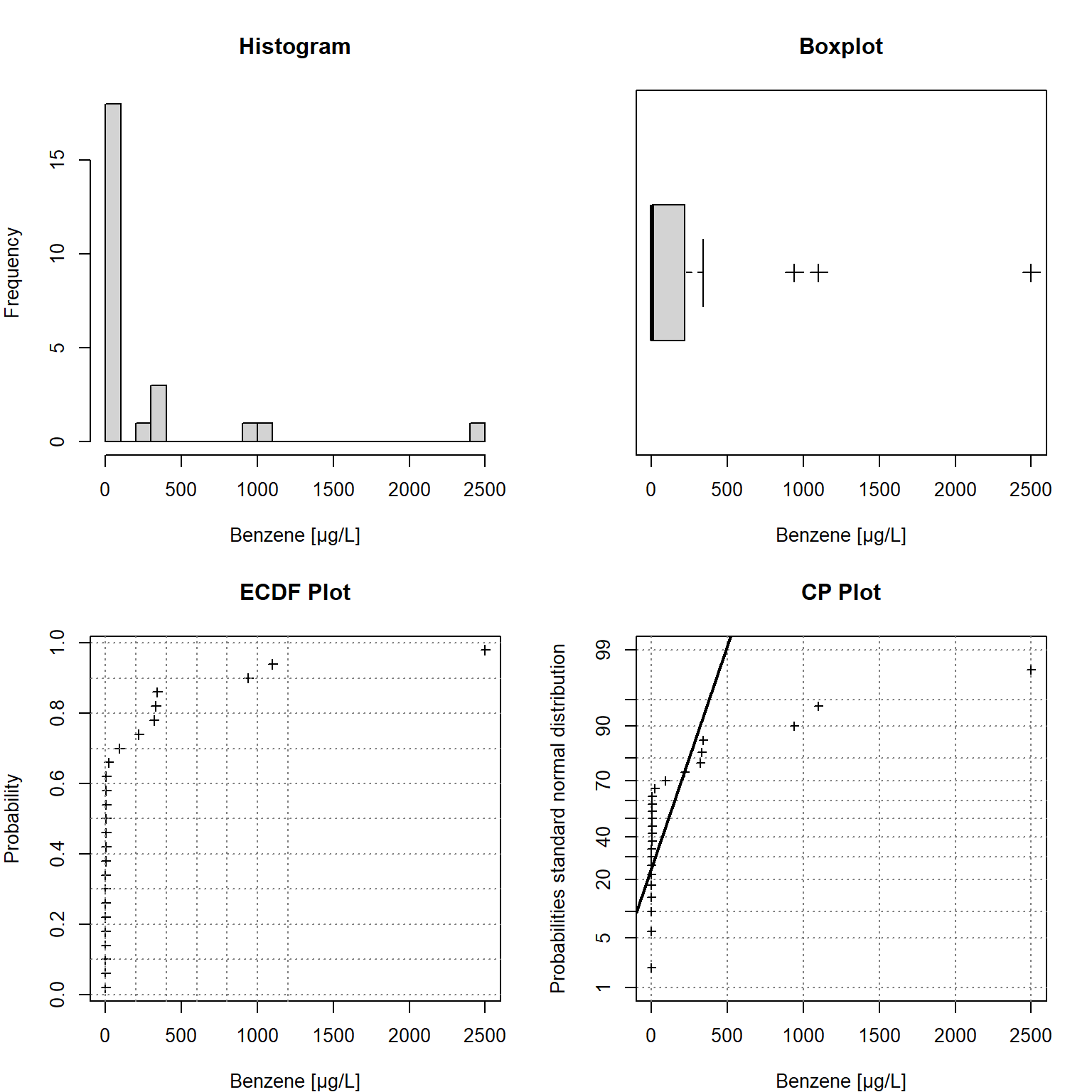
Figure 2: Univariate Statistical Plots

Spatial Data Structure

A plot of each groundwater monitoring well location along with its label is shown in Figure 3. The locations are relatively well-distributed across the site with some localized clustering in the central portion of the site near the eastern boundary. Figure 4 provides a post-plot of the benzene concentration at each monitoring well. The size of each symbol reflects the actual concentration at that location; larger symbols equate to higher concentrations on a log scale. The plot indicates higher benzene concentrations located within the interior of the monitoring well network with lower concentrations along the outer hull of the network.

# Prep data
dat <- datin %>%
  dplyr::select(XCOORD, YCOORD, RESULT, LOCID) %>%
  dplyr::rename(
    x = XCOORD,
    y = YCOORD,
    conc = RESULT,
    locid = LOCID
  )

# Make data geospatial object
coordinates(dat) = ~x+y
proj4string(dat) = CRS(paste0("+init=epsg:", epsg))

# Set plotting window for 2 x 2 plots
par(mar = c(4, 4, 2, 2))

# Plot the locations of each station along with its label
plot(
  coordinates(dat),
  xlim = c(6455350, 6456650),
  pch = "+", col = "red", cex = 1.8,
  asp = 1,
  xlab = "Easting", ylab = "Northing",
  main = NULL #"Groundwater Monitoring Well Locations"
)
grid(lwd = 1.4, col = "grey20")
text(coordinates(dat), labels = dat@data$locid, pos = 4, cex = 0.8)

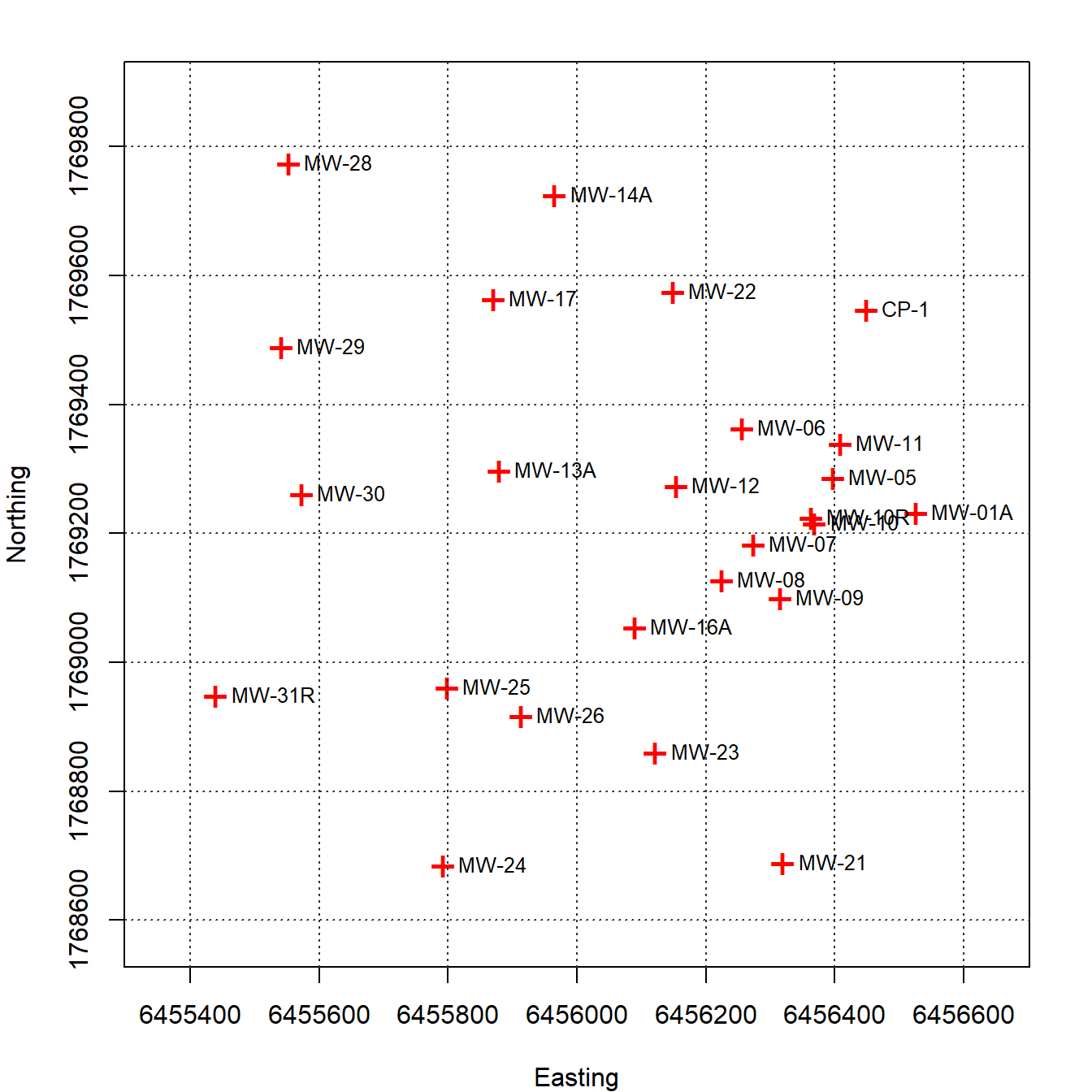
Figure 3: Groundwater Monitoring Well Locations

# Set plotting window for 2 x 2 plots
par(mar = c(4, 4, 2, 2))

# Make a post-plot of concentrations
plot(
  coordinates(dat),
  xlim = c(6455350, 6456650),
  pch = 16, col = "red", asp = 1,
  cex = ifelse(dat@data$conc == 0.1, log(20*dat@data$conc), log(dat@data$conc)),
  #cex = 10*dat@data$conc/max(na.omit(dat@data$conc)),
  xlab = "Easting", ylab = "Northing",
  main = NULL #"Post Plot of Benzene Concentration (µg/L)"
)
text(coordinates(dat), labels = round(dat@data$conc, 2), pos = 2)
grid(lwd = 1.4, col = "grey20")

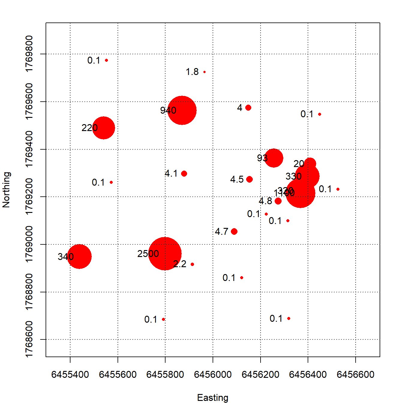
Figure 4: Post Plot of Benzene Concentrations (µg/L)

Results

Ordinary kriging was used to interpolate benzene concentrations in groundwater at the site using the monitoring well data. An omnidirectional variogram was fit to the log-transformed data using an exponential model with a range of 1,000 feet and a sill of 4. Lognormal transformation was used to change the shape of the frequency distribution of the highly skewed distribution of the data. This normalization step reduces data variance and improves the calculation of statistics and weighted averages, such as ordinary kriging estimates. Kriging was conducted using a rectilinear grid 2,390 feet wide (Easting direction) and 1,520 feet long (Northing direction). The grid spacing was 5.975 feet in the x-direction and 3.8 feet in the y-direction. The model domain contained a total of 160,000 nodes.

The interpolated map of benzene concentrations is shown in Figure 5. The exterior boundary of the plume (defined as the 5 µg/L isoconcentration contour) is smooth and appears to be well defined. The smooth, continuous character of the boundary of the plume suggests that sufficient data exist to define the plume although, there are no wells along the western boundary of the plume. The lack of spatial constraint means that concentrations at unsampled locations in ths portion of the plume are being estimated based on extrapolation instead of interpolation. Whereas interpolation is prediction within the extent of the data, extrapolation is prediction outside the extent of the data. Extrapolation is much less reliable than interpolation.

# Setup grid using data extents
delx <- (max(dat@coords[,1]) - min(dat@coords[,1]))*0.6
dely <- (max(dat@coords[,2]) - min(dat@coords[,2]))*0.2

if (expand == 'Y') {
  xb <- round(min(dat@coords[,1]) - delx, -1)
  xe <- round(max(dat@coords[,1]) + delx, -1)
  yb <- round(min(dat@coords[,2]) - dely, -1)
  ye <- round(max(dat@coords[,2]) + dely, -1)
} else {
  xb <- min(dat@coords[,1])
  xe <- max(dat@coords[,1])
  yb <- min(dat@coords[,2])
  ye <- max(dat@coords[,2])
}

xn <- (xe - xb)/nodes
yn <- (ye - yb)/nodes
grid2D <- expand.grid(
  x = seq(xb, xe, xn),
  y = seq(yb, ye, yn)
)
gridded(grid2D) <- ~x+y
proj4string(grid2D) = CRS(paste0("+init=epsg:", epsg))

# Convert from SpatialPixels to SpatialPixelsDataFrame
grid2D.spdf <- SpatialPixelsDataFrame(
  grid2D,
  data = data.frame(grid2D)
)

# Create variogram using omnidirectional variogram
v <- variogram(log10(conc) ~ 1, dat)
v.fit <- fit.variogram(v, vgm(6, "Exp", 1000))
v.fit$psill <- 4
v.fit$range <- 1000

# Kriging
conc.gstat <- quiet(
  krige(log10(conc) ~ 1, dat, grid2D, model = v.fit)
)
pred <- conc.gstat$var1.pred

# Add predictions to spatial pixels object
grid2D.spdf$conc_gstat <- ifelse(pred < log10(5), NA, 10^pred)

# Plot predictions
par(mar = c(1, 1, 1, 1))  # bottom, left, top, right; default is c(5.1, 4.1, 4.1, 2.1)
plot(
  log10(raster(grid2D.spdf['conc_gstat'])),
  col = leg,
  main = NULL, #'Ordinary Kriging',
  axes = FALSE,
  box = FALSE,
  axis.args = axis.ls,
  legend.args = list(
    text = "Result\n(µg/L)", side = 3, font = 2,
    line = 0.2, cex = 0.8
  )
)
points(dat, pch = "+")
text(dat, dat@data$locid, cex = 0.7, pos = 1, col = "black")

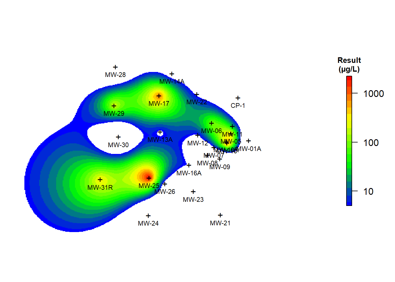
Figure 5: Ordinary Kriging of Benzene Concentrations

Uncertainty in the estimated extent of benzene groundwater concentrations was assessed using SGSIM. Simulation was performed using the ordinary kriging estimator, and the semivariogram model of benzene normal scores. As noted previously, simulation is designed to reproduce the measured level of variability in the sample data for each map of the concentration field while honoring the measured data at their respective locations. Two hundred realizations of the benzene concentration field were generated using the gstat R library (Pebesma and Benedikt 2021). The krige() function of the gstat library can perform conditional simulations by providing one optional argument: nsim, the number of conditional simulations.

The conditional mean and median benzene concentrations based on the post-processing on the 200 simulations are shown in Figure 6. As evident from comparing Figures 5 and 6, the predicted concentrations using ordinary kriging and the E-type estimates of 200 realizations are similar but not identical. Kriging prediction maps smooth out local details of spatial distribution of the variable under study, with small values being overestimated while large values are underestimated, especially in areas with low sampling density (Isaaks and Srivastava 1989). SGSIM techniques, unlike kriging, produce a better picture of reality and eliminate unrealistic smoothing by focusing on the reproduction of global statistics while honoring the original data values (Goovaerts 1997). It is evident that the simulation realizations present more detailed information than the ordinary kriging map. The kriging map is smoothed and does not properly represent the true spatial variation of benzene concentrations in groundwater at the site. Consequently, the local accuracy of the kriging map comes at the cost of a poor reproduction of the spatial pattern in the data. Alternatively, the conditional SGSIM maps present a more realistic reproduction of the spatial pattern in the data.

# Perform simulations
sim <- quiet(
  krige(
    formula = log10(conc) ~ 1, dat,
    grid2D, model = v.fit, 
    nmax = 50, nsim = 200
  )
)

# Process output
sim.mean <- rowMeans(sim@data, na.rm = TRUE)
sim.median <- apply(sim@data, 1, quantile , probs = 0.5, na.rm = TRUE)
sim.exceed <- apply(sim@data, 1, function(x) {
  sum(x > log10(5)) / length(x)
})

# Add predictions to spatial pixels object
grid2D.spdf$sim.mean <- ifelse(sim.mean < log10(5), NA, 10^sim.mean)
grid2D.spdf$sim.median <- ifelse(sim.median < log10(5), NA, 10^sim.median)
grid2D.spdf$sim.exceed <- ifelse(sim.exceed < 0, NA, sim.exceed)

# Plot predictions
par(mar = c(1, 1, 1, 1))  # bottom, left, top, right; default is c(5.1, 4.1, 4.1, 2.1)

# Fist plot
plot(
  log10(raster(grid2D.spdf['sim.mean'])),
  col = leg,
  main = 'SGSIM Mean',
  axes = FALSE,
  box = FALSE,
  axis.args = axis.ls,
  legend.args = list(
    text = "Result\n(µg/L)", side = 3, font = 2,
    line = 0.2, cex = 0.8
  )
)
points(dat, pch = "+")
text(dat, dat@data$locid, cex = 0.7, pos = 1, col = "black")

# Second plot
plot(
  log10(raster(grid2D.spdf['sim.median'])),
  col = leg,
  main = 'SGSIM Median',
  axes = FALSE,
  box = FALSE,
  axis.args = axis.ls,
  legend.args = list(
    text = "Result\n(µg/L)", side = 3, font = 2,
    line = 0.2, cex = 0.8
  )
)
points(dat, pch = "+")
text(dat, dat@data$locid, cex = 0.7, pos = 1, col = "black")

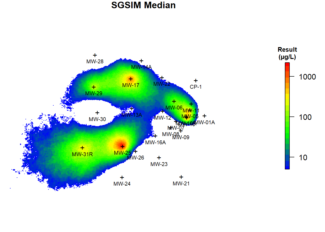
Figure 6: Conditional Mean and Median Benzene Concentrations Using SGSIM

Figure 7 presents the probabistic summary for benzene exceeding 5 µg/L in groundwater that was generated from the ensemble of simulated benzene concentration fields. In the figure, the color-scale values represent the probability of exceeding 5 µg/L, rather than indicating estimates of concentration. Looking at Figure 7, it can be determined that the probability of exceeding 5 µg/L is very high in the central portion of the site. Conversely, the probability of exceeding 5 µg/L is rather low in the eastern portion of the site. Areas of highest uncertainty are those within the 0.4 to 0.6 probability contour region, shown in the map as chartreuse. These areas are primarily located in the western portion of the site.

# Plot predictions
par(mar = c(1, 1, 1, 1))  # bottom, left, top, right; default is c(5.1, 4.1, 4.1, 2.1)

# Exceedance
plot(
  raster(grid2D.spdf['sim.exceed']),
  col = leg,
  main = paste0('Probability Exceeding 5 ', '\u03bc', 'g/L'),
  axes = FALSE,
  box = FALSE,
  legend.args = list(
    text = "Probability", side = 3, font = 2,
    line = 0.2, cex = 0.8
  )
)
points(dat, pch = "+")
text(dat, dat@data$locid, cex = 0.7, pos = 1, col = "black")

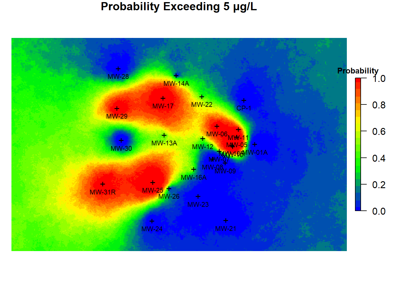
Figure 7: Benzene Probability of Exceedance Map Using SGSIM

Conclusions

Geostatistical simulation provides a useful tool for examining the uncertainty inherent in groundwater monitoring well networks. Geostatistical simulation is an alternative approach to kriging estimation and consists of generating multiple realizations of the spatial distribution of contamination, providing a visual and quantitative measure of spatial uncertainty. A simulated map preserves the correlation structure, whereas kriging smooths (i.e., reduces variance) the predicted concentrations. Simulation attempts to capture the statistical characteristics of the data in a set of alternative stochastic realizations. which can be used to help understand data uncertainty. The set of alternative realizations generated with geostatistical simulation provides a degree of uncertainty about the spatial prediction, which can be used to estimate reliable probability maps. Geostatistical simulation is increasingly preferred to kriging for characterization of uncertainty for decision and risk analysis rather than producing the best unbiased prediction of unsampled location as is done with kriging (Deutsch and Journel 1998).

References

Bivand, R., T. Keitt, and B. Rowlingson. 2021. Rgdal: Bindings for the Geospatial Data Abstraction Library. https://CRAN.R-project.org/package=rgdal

Deutsch, C.V. 2002. Geostatistical Reservoir Modeling. Oxford University Press, New York, 2002.

Deutsch, C.V. and A.G. Journel. 1998. GSLIB Geostatistical Software Library and User’s Guide, Second Edition. Oxford University Press, New York.

Goovaerts, P. 1997. Geostatistics for Natural Resource Evaluation. Oxford University Press, New York.

Goovaerts, P. 1999. Geostatistics in soil science: state-of-the-art and perspectives. Geoderma. 89, 1-45.

Hijmans, R. J. 2020. Raster: Geographic Data Analysis and Modeling. https://rspatial.org/raster.

Isaaks, E.H. and R.M. Srivastava. 1989. An Introduction to Applied Geostatistics. New York: Oxford University Press.

Kaplan, E.L. and O. Meier. 1958. Nonparametric Estimation from Incomplete Observations. Journal of the American Statistical Association, 53, 457-481.

Krige, D. G. 1951. A statistical approach to some basic mine valuation problems on the Witwatersrand. Journal of the Chemical, Metallurgical and Mining Society of South Africa, 52, 119-139.

Matheron, G. 1963. Principles of Geostatistics. Economic Geol., 58, 1246-1268.

Pebesma, E. and G. Benedikt. 2021. Gstat: Spatial and Spatio-Temporal Geostatistical Modelling, Prediction and Simulation. https://github.com/r-spatial/gstat/.

R Core Team. 2021. R: A Language and Environment for Statistical Computing. R Foundation for Statistical Computing, Vienna, Austria. http://www.R-project.org.

Ribeiro, Jr., P.J., P.J. Diggle, O. Christensen, M. Schlater, R. Bivand, and B. Ripley. 2020. geoR: Analysis of Geostatistical Data. https://cran.r-project.org/web/packages/geoR/index.html.

Zanon, S. and O. Leuangthong. 2004. Implementation aspects of sequential simulation. Geostatistics Banff, 1, 543-550.