Introduction

Costs for long-term groundwater monitoring (LTM) represent a significant, persistent, and growing burden for private entities and government agencies responsible for environmental remediation projects. LTM programs typically require extensive data collection and analyses, some of which are often irrelevant to the objectives of the monitoring program. The costs for excessive data collection are compounded by the costs of data processing, management, review, and archiving as well as for the preparation of a periodic LTM report.

Many existing LTM well networks are either developed during site characterization activities or in the initial stages of groundwater remediation. As a consequence, these well networks do not reflect changes in site conditions, resulting in too many wells being sampled too often. Wells that provide redundant information or that do not meet the objectives of the LTM program are unnecessary and should be eliminated from the monitoring program. Optimization of LTM networks offers an opportunity to improve the cost-effectiveness of groundwater monitoring by ensuring objectives are achieved with an appropriate level of effort. Optimization may identify redundancies in the monitoring program that can be removed or inadequacies that may require changes in the monitoring program to protect against potential impacts to the environment. The difficulty of finding optimal well network designs is that a quantitative criterion is often a priori not present.

This factsheet is the last of three factsheets that uses geostatistical methods to spatially optimize groundwater monitoring well networks. The first factsheet presented a simple approach to identify where new wells should be located or which well locations should be removed such that the operational value of the monitoring network is maximized. The second factsheet described the use of Sequential Gaussian Simulation conditioned on measured groundwater concentration data to assess spatial variability in the predicted distribution of contamination. This third and last factsheet performs geospatial optimization of a groundwater monitoring well network with the objective of minimizing the number of sample locations needed to represent the plume, subject to the constraint that the characteristics of the plume remain comparable. The objective of these three factsheets is to help streamline and optimize existing or planned LTM well networks while maintaining or increasing monitoring effectiveness.

Methodology

Geostatistical data are data that could in principle be measured anywhere, but that typically come as measurements at a limited number of observation locations. The interest in collecting these data is usually in inference of aspects of the variable that have not been measured, such as maps of the estimated values, exceedence probabilities, or estimates of aggregates over given regions. Geostatistical techniques based on semivariogram modeling and kriging are generally used to eliminate spatially redundant sampling locations. These locations contribute little additional information regarding plume characterization because of their spatial correlation with other monitoring wells. In practice, geospatial optimization techniques are often applied to LTM programs because these programs typically provide well-defined spatial coverage of the area monitored, and have been implemented for a period of time sufficient to generate a relatively comprehensive monitoring history.

Well Network Optimization Methodology

The main objective of groundwater monitoring is to provide an accurate assessment of groundwater quality over space and time. Interpolated maps are used to assess whether a plume of contaminated groundwater exists and, if so, the extent and characteristics of the contaminated groundwater. Changes in the interpolated maps and/or concentration patterns over time can indicate either improvement or decline in groundwater quality across the plume area. Spatial optimization assumes that well locations are spatially redundant if nearby wells offer similar information about the underlying plume and removal would not significantly change an interpolated map of the plume.

For each contaminant of concern, an initial plume map is generated using all of the current groundwater monitoring wells. Then, the number of wells used to generate the plume map is reduced iteratively until similar plume maps are obtained, but using a smaller set of wells. The underlying assumption is that the initial plume map, based on all existing wells, is the best possible representation of the plume because it is generated using the largest amount of available data. Redundant locations can be eliminated without significantly degrading the character of the resulting plume generated with the reduced data set. The character of the plume is defined by three metrics: plume area, plume mass, and visual appearance. Each of these metrics should remain approximately constant from one iteration to the next.

In effect, the procedure is an optimization of the monitoring well network with the objective of minimizing the number of sample locations needed to represent the plume, subject to the constraint that the three metrics remain comparable. Comparability of plume area and plume mass can be evaluated quantitatively while invariance of plume appearance is evaluated subjectively. When essential wells are eliminated during the iterative evaluation to identify redundant locations, the visual impact on plume boundary is obvious, as are the impacts on quantitative measurements of the plume such as area and mass.

Interpolation over the spatial area of interest is performed using ordinary kriging. Kriging, developed by the South African mining engineer D. G. Krige (1951) and latter formalized by the French geologist and statistician Georges Matheron (1963), is a family of estimators used to interpolate spatial data. Kriging is an interpolation technique that calculates a concentration at an unknown location through a weighted average of known points within a data-specific neighborhood (Isaaks and Srivastava 1989). Variography is used to calculate the weights, thereby incorporating the spatial correlation within the interpolation. Ordinary kriging (Isaaks and Srivastava 1989; Gooevaerts 1997) is one of the simplest forms of kriging. It assumes a constant but unknown mean over the search neighborhood.

Interpolation, plume visualization, and estimation of plume metrics were performed using the gstat (Pebesma and Benedikt 2021) and sp (Bivand et al. 2013) libraries run within the statistical software R version 4.1.1 (R Core Team 2021).

Parameters

Several libraries, functions, and parameters are required to perform the spatial optimization.

# Load libraries
library(dplyr)
library(sp)

# Load functions
source('functions/SumStats.R')

# Set options so no scientific notation
epsg <- 32042
options(scipen = 999)

Data

The data consist of trichloroethene (TCE) concentrations measured during a single sampling event. Results are given in µg/L. The data consist of a mixture of detects and non-detects. The non-detects have been assigned a value of 0.05 µg/L, which is one-half the detection limit. The groundwater monitoring well network corresponding to the TCE concentration data consists of 86 groundwater monitoring wells installed in an shallow groundwater system, located within deltaic sediments deposited as interbedded silt, clay, and sand layers on a terraced, north-facing escarpment.

The structure of the data is shown below and consists of seven variables. Variables include well id, parameter name, measurement result, units of measure, whether the result is a detect (“Y”) or non-detect (“N”), and geographical coordinates (given in feet) for each well.

# Load data
datin <- read.csv('data/OU4TCE_LastResult.csv', header = T)

# View structure of data
str(datin)

## 'data.frame':	86 obs. of  7 variables:
##  $ LOCID : chr  "U4-001" "U4-002" "U4-006" "U4-008" ...
##  $ PARAM : chr  "TCE" "TCE" "TCE" "TCE" ...
##  $ DETECT: chr  "Y" "N" "Y" "Y" ...
##  $ RESULT: num  1500 0.05 200 810 320 2 210 0.05 0.05 0.05 ...
##  $ UNITS : chr  "ug/L" "ug/L" "ug/L" "ug/L" ...
##  $ XCOORD: num  1863922 1862667 1863633 1863755 1863745 ...
##  $ YCOORD: num  297588 297819 297705 297846 297852 ...

Summary Statistics

Summary statistics of TCE concentrations are shown below. Of the 86 sample results, 53 samples (61.6%) had detectable concentrations. The minimum and maximum concentrations are <0.1 and 12,000 µg/L, respectively. The mean concentration is 386 µg/L with a median concentration of 4.7 µg/L, a standard deviation of 1,738 µg/L, and a coefficient of variation (CV) of 4.5. Univariate statistical plots are shown in Figure 1. The plots include a histogram in the upper left window, an empirical cumulative density function (ECDF) plot in the lower left window, a box plot in the upper right window, and a cumulative probability (CP) plot in the lower right window. As shown in the plots, the data are strongly right-skewed.

# Get summary statistics and transpose
zz <- SumStats(datin, rv = 2)
names <-  zz[,1]  # keep 1st column
zz.T <- data.frame(as.matrix(t(zz[,-1])))  # transpose everything but 1st column
colnames(zz.T) <- names  # assign 1st column as column names
zz.T

##              TCE
## Obs        86.00
## Dets       53.00
## DetFreq    61.63
## MinND       0.05
## MinDET      0.53
## MaxND       0.05
## MaxDet  12000.00
## Mean      386.47
## Median      4.70
## SD       1737.93
## CV          4.50

# Load data
TCE <- datin[,"RESULT"]
n <- length(TCE)

# Set plotting window for 2 x 2 plots
par(mfcol = c(2, 2), mar = c(4, 4, 4, 2))

# Plot 1. Histogram
hist(
  TCE,
  breaks = 25,
  main = "",
  xlab = "TCE [µg/L]",
  ylab = "Frequency",
  cex.lab = 1
)
title("Histogram")

# Plot 2. Empirical Cumulative Density Function Plot
plot(
  sort(TCE),
  ((1:n) - 0.5)/n,
  pch = 3, cex = 0.8,
  main = "",
  xlab = "TCE [µg/L]",
  ylab = "Probability",
  cex.lab = 1
)
abline(h = seq(0, 1, by = 0.1), lty = 3, col = gray(0.5))
abline(v = seq(0, 1200, by = 200), lty = 3,col = gray(0.5))
title("ECDF Plot")

# Plot 3. Boxplot
boxplot(
  TCE,
  horizontal = T,
  xlab = "TCE [µg/L]",
  cex.lab = 1, pch = 3, cex = 1.5
)
title("Boxplot")

# Plot 4. Quantile-Probability Plot
StatDA::qpplot.das(
  TCE,
  qdist = qnorm,
  xlab = "TCE [µg/L]",
  ylab = "Probabilities standard normal distribution",
  pch = 3, cex = 0.7, cex.lab = 1,
  logx = FALSE
)
title("CP Plot")

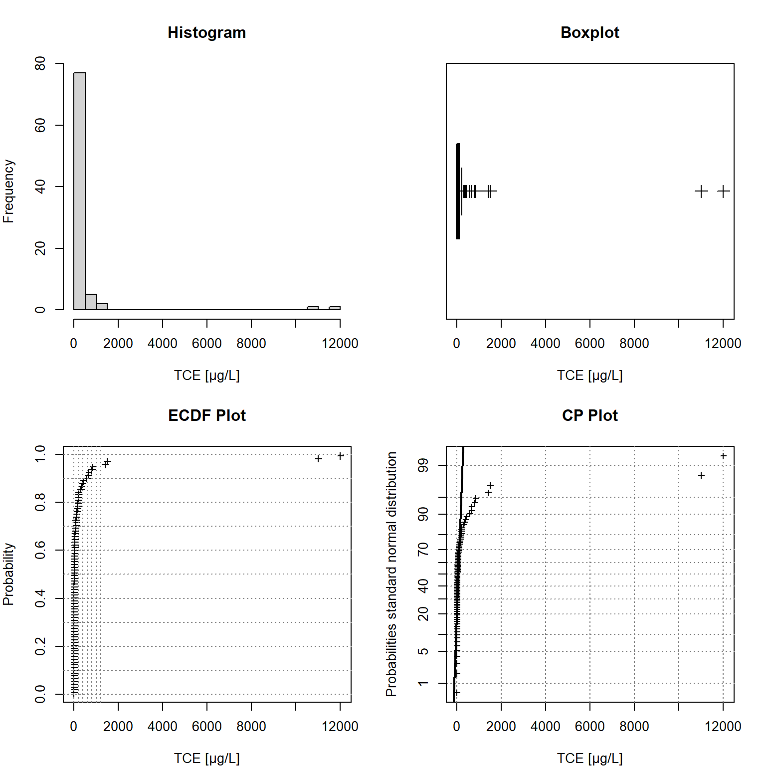
Figure 1: Univariate Statistical Plots

Spatial Data Structure

A plot of each groundwater monitoring well location along with its label is shown in Figure 2. The locations are relatively well-distributed across the site with some localized clustering in the southeastern portion of the site near the suspected source zone. Groundwater flow in the shallow aquifer is to the north. Figure 3 provides a post-plot of the TCE concentration at each monitoring well. The size of each symbol reflects the actual concentration at that location; larger symbols equate to higher concentrations on a log scale. The plot indicates higher TCE concentrations located in the southeastern portion of the site with lower concentrations along the outer hull of the monitoring well network.

# Prep data
dat <- datin %>%
  dplyr::select(XCOORD, YCOORD, RESULT, LOCID) %>%
  dplyr::rename(
    x = XCOORD,
    y = YCOORD,
    conc = RESULT,
    locid = LOCID
  )

# Make data geospatial object
coordinates(dat) = ~x+y
proj4string(dat) = CRS(paste0("+init=epsg:", epsg))

# Set plotting window for 2 x 2 plots
par(mar = c(4, 4, 2, 2))

# Plot the locations of each station along with its label
plot(
  coordinates(dat),
  pch = "+", col = "red", cex = 1.8,
  asp = 1,
  xlab = "Easting", ylab = "Northing",
  main = NULL #"Groundwater Monitoring Well Locations"
)
grid(lwd = 1.4, col = "grey20")
text(coordinates(dat), labels = dat@data$locid, pos = 4, cex = 0.6)

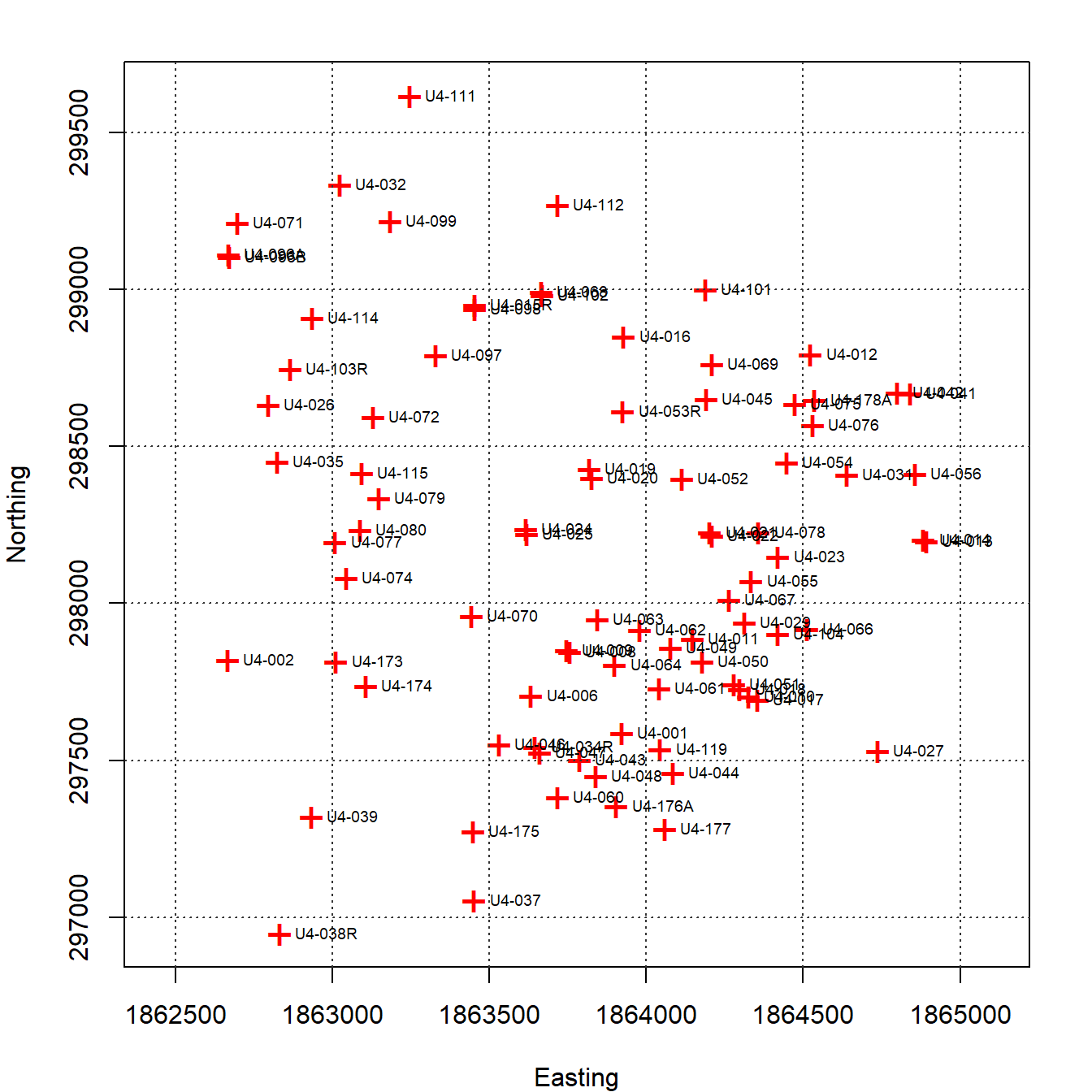
Figure 2: Groundwater Monitoring Well Locations

# Set plotting window for 2 x 2 plots
par(mar = c(4, 4, 2, 2))

# Make a post-plot of concentrations
plot(
  coordinates(dat),
  pch = 16, col = "red", asp = 1,
  cex = ifelse(dat@data$conc < 23, 0.5, log(0.1*dat@data$conc)),
  #cex = 10*dat@data$conc/max(na.omit(dat@data$conc)),
  xlab = "Easting", ylab = "Northing",
  main = NULL #"Post Plot of TCE Concentration (µg/L)"
)
text(coordinates(dat), labels = round(dat@data$conc, 2), pos = 2, cex = 0.6)
grid(lwd = 1.4, col = "grey20")

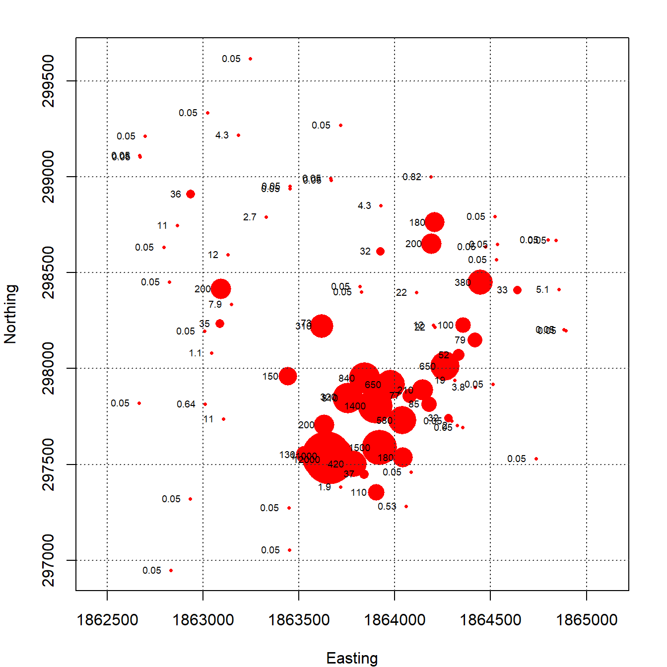
Figure 3: Post Plot of TCE Concentrations (µg/L)

Monitoring Well Network Optimization Results

Geospatial optimization of the LTM well network shown in Figure 2 was performed using the most recent TCE concentration data collected from the 86 wells. The analysis was conducted to evaluate whether all wells currently being monitored are needed to provide an accurate assessment of groundwater quality. Optimization included the following steps.:

1. Generate an initial plume map by kriging data collected from all groundwater monitoring wells.

2. Assign numerical weights to wells based on their contribution to delineating the areal extent of the plume and estimating the plume mass.

3. Iteratively remove wells, starting with the lowest weight well, and re-estimate the plume map for each subset of data.

4. Assess if the newly estimated plume maps provide an acceptable representation of current conditions based on:

   a. A change of 10 percent or less for the estimated plume area b. A change of 10 percent or less for the estimated plume mass

5. Retain wells if their removal from the monitoring network results in an unacceptable change in the representation of plume conditions.

6. Generate a final plume map using data collected from the optimized subset of wells.

Interpolated contours of groundwater TCE concentrations using existing analytical data for all monitoring wells in the LTM network are shown in Figure 4. The wells for this initial plume map, or base map, are shown as circles, where the color of the circle is correlated to the most recent concentration of TCE reported for that well. The concentrations have been assigned to logarithmic intervals, where the first interval given as dark blue represents concentrations below 5 µg/L. The color-scale values for the plume contour intervals are the same as those used for the well concentrations.

The appearance of the TCE plume obtained by using the initial set of wells suggests that the data are an appropriate starting point for subsequent analysis of the monitoring network. The exterior boundary of the plume (defined as the 5-µg/L isoconcentration contour) is smooth and well defined. The smooth, continuous character of the boundary of the plume indicates that sufficient data exist to define the plume using interpolation rather than extrapolation.

Figure 5 presents the interpolated contours of groundwater TCE concentrations using the optimized subset of monitoring wells. The color-scale used in this final, optimized plume map is the same as that used for creating the base map. The spatial extent of TCE contamination, defined as the region bounded by the 5-µg/L isoconcentration contour, for the optimized plume map is essentially the same as that of the corresponding base map, where data from all wells were used in the interpolation. The interior isoconcentration contours (defined as greater than 5 µg/L) also are similar on the optimized and base maps.

Changes in the quantitative metrics using the optimized well network are within 10 percent of those estimated for the base plume condition. The area within the 5-µg/L isoconcentration contour of the initial base plume, using all of the wells, is 39.3 acres. The area within the 5-µg/L isoconcentration contour of the final plume, using the optimized list of wells, is 41.2 acres. This represents a difference of 4.8%. The dissolved mass of TCE in the base plume is 58.2 kilograms (kg) compared to 61.1 kg in the final plume. This represents an increase in the estimated plume mass of 5.0%.

These results indicate that spatially redundant wells can be eliminated from the LTM well network without significantly degrading the character of the resulting plume generated with the reduced data set. Of the 86 wells in the LTM network, 39 wells were identified as spatially redundant based on the geospatial analysis. These spatially redundant wells are shown with magenta crosses on the final optimized plume map in Figure 5. The number of wells in the optimized monitoring network represents a reduction of approximately 45% from the initial number of wells used to monitor groundwater at the site.

Figure 4: TCE Plume Map Using All Monitoring Wells

Figure 5: TCE Plume Map Using Optimized Subset of Monitoring Wells

Conclusions

Redundancy in the number and placement of monitoring wells (spatial redundancy) generally is present in most LTM programs. Monitoring networks with optimally located groundwater monitoring wells collecting prerequisite data provide insights for strategic planning and decision making. An optimized monitoring well network can significantly reduce site life-cycle costs without losing information critical to protecting human health and the environment. This is particularly important for sites with lengthy remedial timeframes. The efficiency of a monitoring program is considered to be optimal if it is effectively achieving its objectives at the lowest total cost with the fewest possible number of monitoring locations.

Most current approaches to optimizing groundwater monitoring well networks typically rely on professional engineering judgment as opposed to statistical logic. Geostatistical techniques provide a more robust method to assess the adequacy of a monitoring well network based on the spatial characteristics of the collected data. Successful application is directly dependent upon the amount and quality of the available data. The maturity of the monitoring program, the number of wells, and the longevity of the data record needs to be considered prior to performing optimization. The data need to provide sufficient statistical basis to conduct a groundwater monitoring optimization study. In addition to acquiring and processing the data, it is important to evaluate the data in terms of quality and comparability. The defensibility and usability of the data should support statistical analysis. Because there may be other considerations that are best addressed through a qualitative evaluation, final recommendations for optimization should be qualitatively reviewed to assess the impacts of site hydrogeologic characteristics and stakeholder considerations.

References

Bivand, R.S., E. Pebesma, and V. Gomez-Rubio. 2013. Applied Spatial Data Analysis with R, Second edition. New York: Springer.

Goovaerts, P. 1997. Geostatistics for Natural Resource Evaluation. Oxford University Press, New York.

Isaaks, E.H. and R.M. Srivastava. 1989. An Introduction to Applied Geostatistics. New York: Oxford University Press.

Krige, D. G. 1951. A statistical approach to some basic mine valuation problems on the Witwatersrand. Journal of the Chemical, Metallurgical and Mining Society of South Africa, 52, 119-139.

Matheron, G. 1963. Principles of Geostatistics. Economic Geol., 58, 1246-1268.

Pebesma, E. and G. Benedikt. 2021. Gstat: Spatial and Spatio-Temporal Geostatistical Modelling, Prediction and Simulation. https://github.com/r-spatial/gstat/.

R Core Team. 2021. R: A Language and Environment for Statistical Computing. R Foundation for Statistical Computing, Vienna, Austria. http://www.R-project.org.