Groundwater Statistics Using trendMK
A Brief Introduction to R
By Charles Holbert
March 13, 2022
Introduction
This is a brief tutorial on groundwater statistics using the R package trendMK. R is an open-source programming language for statistical computing and data visualization (R Core Team 2021). R has become the preferred computing environment for a large part of the statistical community. R is increasingly being used as an industry standard in the realm of data analytics, also known as “data science.” R has a package system that makes it extremely easy for people to add their own functionality that is relatively indistinguishable from the base R functionality.
The trendMK package is used for the graphical and statistical analyses of environmental data, with a focus on analyzing chemical concentrations and physical parameters, usually in the context of mandated environmental monitoring and reporting. The trendMK package includes procedures for calculating summary statistics for censored and non-censored data sets; parametric and nonparametric tests for statistical outliers; regression analysis; tests for trend detection; estimates of remedial timeframes based on first-order attenutaion rate constants; and various graphical presentations of data. The trendMK package is designed to analyze data sets containing many sampling locations and monitoring constituents.
This package is free software and can be redistributed and/or modified under the terms of the GNU GPL 3 as published by the Free Software Foundation. This package is distributed in the hope that it will be useful, but without any warranty; without even the implied warranty of merchantability of fitness for a particular purpose.
Packages
In R, the fundamental unit of reproducible code is the package, also referred to as a library. A package bundles together code, data, and documentation into a well-defined format that is easy to share with others. There are a set of standard (or base) packages that are automatically available as part of the R installation. Base packages contain the basic functions that allow R to work, and enable standard statistical and graphical functions to be performed. However, for specific types of actions, additional packages that others have created often need to be installed. R packages are the best way to distribute R code and documentation. These packages can be downloaded from a variety of sources but the most popular are CRAN, Bioconductor and GitHub. CRAN is the official repository for user-contributed R packages. Bioconductor provides packages oriented towards bioinformatics and GitHub is a website that hosts git repositories for all sorts of software and projects (not just R).
Packages can be installed within the R console window by running install.packages(“package name”). Once installed a package is not immediately available for use. To use a package, it needs to be loaded using the library() function. We will be using several packages as part of this example. Let’s load the packages using the code shown below.
# Load libraries
library(dplyr)
library(tidyr)
library(trendMK)
library(knitr)
library(kableExtra)
library(formattable)
Data
For this example, the data consist of four volatile organic compounds (VOCs) measured in groundwater samples collected over a 15-year period from 31 groundwater monitoring wells. The VOCs are tetrachloroethene, trichloroethene, cis-1,2-dichloroethene, and vinyl choride.
First, we will create a parameter list using the exact names that are contained in our data file. We then will create a list of cleanup values in the same order as the parameter names. Finally, we combine the parameter list with the list of cleanup values into a single data frame named cleanup_levels. A data frame is the most common way of storing data in R and, generally, is the data structure most often used for data analyses. Under the hood, a data frame is a list of equal-length vectors. The clean_up levels data frame will be used when we calculate first-order attenuation rate constants and estimate remedial timeframes for each VOC and monitoring well.
# Read in parameter list
params <- c(
  'Tetrachloroethene',
  'Trichloroethene',
  'cis-1,2-Dichloroethene',
  'Vinyl Chloride'
)

# Create list with cleanup levels in same order as parameter names
level <- c(5, 5, 70, 2)

# Combine parameter and cleanup lists into data frame
cleanup_levels <- data.frame(params, level)
str(cleanup_levels)
## 'data.frame':	4 obs. of  2 variables:
##  $ params: chr  "Tetrachloroethene" "Trichloroethene" "cis-1,2-Dichloroethene" "Vinyl Chloride"
##  $ level : num  5 5 70 2
We see that our clean_up_levels data frame contains the four compounds (Tetrachloroethene, Trichloroethene, cis-1,2-Dichloroethene, and Vinyl Chloride) with their corresponding clean values of 5, 5, 70, and 2 \(\mu\)g/L, respectively.
While we are defining parameters, let’s create a minimum and maximum date variable. These variables can be used to subset, or filter, the data in case we would like to rerun the analysis using a different time period.
# Set min and max date for subsettting data
mindate <- as.POSIXct('1/1/1970', format = '%m/%d/%Y')
maxdate <- as.POSIXct('1/1/2022', format = '%m/%d/%Y')
We have set the minimum date to 1970-01-01 and the maximum date to 2022-01-01. These dates encompass all the data. However, if we decide to analyze the data using a different time period, all we have to do is change these dates accordingly and then rerun the code.
Now that we have created our parameters, let’s load the data. While there are R packages designed to access data from Excel spreadsheets, I find it easier to save the data as a comma-delimited file (csv) and then use R’s built in functionality to read and manipulate the data. We will use the built in read.csv() function, which reads the data in as a data frame. We will assign the data frame to a variable using R’s assignment operator <- so that it is stored in R’s memory. There is a general preference among the R community for using <- for assignment. However, many people use = for assignment.
# Read data from comma-delimited file
datin <- read.csv('data/exdata.csv', header = T)
Now that we have our data read into memory, let’s prepare the data for analysis using the mutate() and filter() functions from the dplyr package. First, we will let R know the format of the sample dates that are contained in our data. The format = ‘%m/%d/%Y’ tells R that the format of the sample dates are calendar dates given as m/d/yyyy. Next, let’s add a column to our data frame called RESULT2 that assigns one-half the method detection limit (MDL) to the non-detects, which are identified using “Y” for detects and “N” for non-detects in the DETECTED column. The RESULT2 values are only needed for regression analysis and estimating first-order attenuation rates constants and remedial timeframes.
Note that we are using the pipe operator %>% that comes from the magrittr package and that is automatically loaded with the dplyr package. It takes the output of one function and passes it into another function as an argument. This allows us to link a sequence of steps used in the data processing and analysis. The purpose of the pipe operator is to help you write code in a way that is easier to read and understand.
Let’s filter the data by the parameter names and the minimum and maximum date variables. Note that the data frame resulting from filter() will retain all the levels of a factor from the original data frame. We use R’s droplevels() function to remove unused factor levels. Let’s make the PARAM variable an ordered factor so that our results will be order in the same manner as the parameter list we established at the beginning of this tutorial. If we did not do this, the results and output would be order alphabetically. Finally, let’s sort the data frame by parameter name (PARAM), well name (LOCID), and sample date (LOGDATE).
Now, let’s inspect the general structure of the data frame using the str() function. We see that our data are comprised of 3,703 observations with 14 variables. LOGDATE is a calendar date, PARAM is an ordered factor, and the remaining variables are either characters or numbers.
# Prep data
dat <- datin %>%
  mutate(
    LOGDATE = as.POSIXct(LOGDATE, format = '%m/%d/%Y'),
    RESULT2 = ifelse(DETECTED == 'Y', RESULT, 0.5*MDL)
  ) %>%
  filter(
    PARAM %in% params &
    LOGDATE >= mindate &
    LOGDATE <= maxdate
  ) %>%
  droplevels()

# Make parameters ordered factor
dat$PARAM <- factor(dat$PARAM, ordered = TRUE, levels = params)

# Sort by parameter, locid, and then date
dat <- dat[with(dat, order(PARAM, LOCID, LOGDATE)), ]
str(dat)
## 'data.frame':	3703 obs. of  14 variables:
##  $ LOCID     : chr  "MW01" "MW01" "MW01" "MW01" ...
##  $ SACODE    : chr  "N" "N" "N" "N" ...
##  $ LOGDATE   : POSIXct, format: "2009-02-26" "2009-04-13" ...
##  $ MATRIX    : chr  "WG" "WG" "WG" "WG" ...
##  $ METHOD    : chr  "SW8260" "SW8260" "SW8260" "SW8260" ...
##  $ CAS       : chr  "127-18-4" "127-18-4" "127-18-4" "127-18-4" ...
##  $ PARAM     : Ord.factor w/ 4 levels "Tetrachloroethene"<..: 1 1 1 1 1 1 1 1 1 1 ...
##  $ DETECTED  : chr  "Y" "Y" "Y" "Y" ...
##  $ RESULT    : num  1540 1840 1520 267 169 24.9 1850 1440 166 880 ...
##  $ MDL       : num  9.94 19.9 9.94 9.94 7.96 0.398 7.96 19.9 1.99 3.98 ...
##  $ RL        : num  25 50 25 25 20 1 20 50 5 10 ...
##  $ UNITS     : chr  "µg/L" "µg/L" "µg/L" "µg/L" ...
##  $ QUALIFIERS: chr  "" "" "" "" ...
##  $ RESULT2   : num  1540 1840 1520 267 169 24.9 1850 1440 166 880 ...
Data Structure
After preparing the data for analysis, I like to inspect the data to ensure the variables are as expected. The dfSummary() function in the R package summarytools can be used to provide a quick graphical presentation of the data as shown below. The dfSummary() function creates a summary table with statistics, frequencies, and graphs for all variables in a data frame. The information displayed is type-specific (character, factor, numeric, date) and also varies according to the number of distinct values.
Items to inspect are consisteny in the naming conventions used for the character variables. R is case sensitive, so Tetrachloroethene and tetrachlorothene are different variables. Review the summary table shown below to help ensure well names, parameter names, and units are using a consistent naming convention. For instance, units of \(\mu\)g/L and \(\mu\)g/l are different and may affect the results obtained from the statistical analysis.
# View graphical structure of data
library(summarytools)
print(
  dfSummary(
    dat,
    varnumbers   = FALSE,
    valid.col    = FALSE,
    style        = 'grid',
    plain.ascii  = FALSE,
    headings     = FALSE,
    graph.magnif = 0.8
  ),
#  max.tbl.height = 600,
  footnote = NA,
  method = 'render'
)
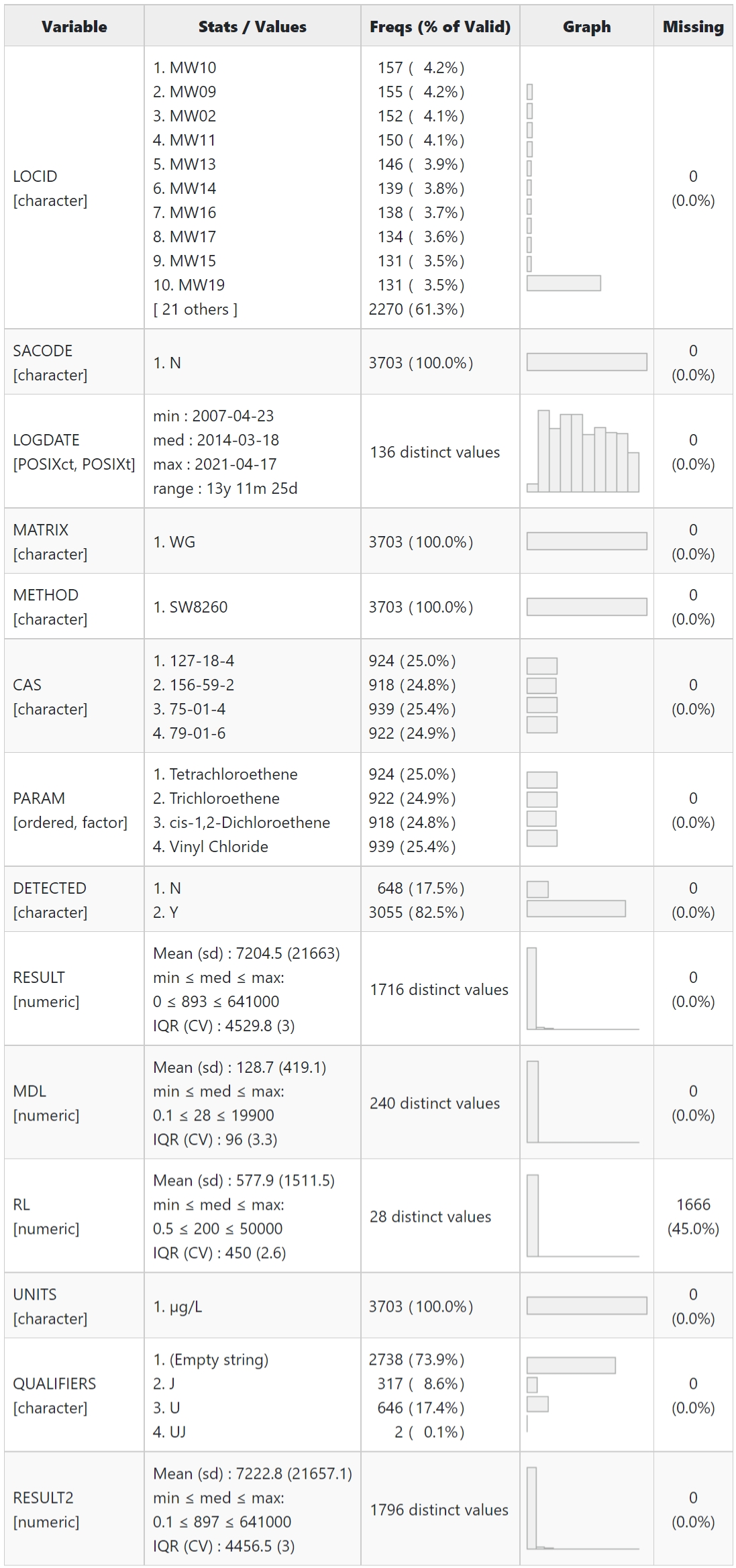
Note that the RL field has 45% missing values. Let’s see if there are missing RL’s for results listed as non-detect. We see below there are no missing RLs for results listed as non-detect.
length(subset(dat, DETECTED == 'N' & is.na(RL))$RESULT)
## [1] 0
Let’s inspect the samples with trace concentrations of one of the VOCS, meaning that the result is less than the reporting limit (RL) and has been flagged with a “J” data qualifier. We see that of the 317 results with a “J” flag, there are 105 that have a result less than the RL. We can use the head() function to inspect the first six rows of the subsetted data and pipe that to the kableExtra package to create a simple table.
length(subset(dat, QUALIFIERS == 'J')$RESULT)
## [1] 317
length(subset(dat, QUALIFIERS == 'J' & RESULT < RL)$RESULT)
## [1] 105
# Inspect J-flag data
head(subset(dat, QUALIFIERS == 'J' & RESULT < RL)) %>%
  kbl(row.names = FALSE) %>%
  kable_classic(full_width = F, font_size = 11, html_font = "Cambria")
| LOCID | SACODE | LOGDATE | MATRIX | METHOD | CAS | PARAM | DETECTED | RESULT | MDL | RL | UNITS | QUALIFIERS | RESULT2 |
|---|---|---|---|---|---|---|---|---|---|---|---|---|---|
| MW04 | N | 2020-04-24 | WG | SW8260 | 127-18-4 | Tetrachloroethene | Y | 3.28 | 2.90 | 5 | µg/L | J | 3.28 |
| MW06 | N | 2021-04-16 | WG | SW8260 | 127-18-4 | Tetrachloroethene | Y | 19.40 | 10.00 | 20 | µg/L | J | 19.40 |
| MW01 | N | 2009-08-25 | WG | SW8260 | 79-01-6 | Trichloroethene | Y | 15.90 | 8.97 | 20 | µg/L | J | 15.90 |
| MW02 | N | 2009-02-25 | WG | SW8260 | 79-01-6 | Trichloroethene | Y | 3670.00 | 2240.00 | 5000 | µg/L | J | 3670.00 |
| MW03 | N | 2009-02-26 | WG | SW8260 | 79-01-6 | Trichloroethene | Y | 1670.00 | 897.00 | 2000 | µg/L | J | 1670.00 |
| MW03 | N | 2009-11-05 | WG | SW8260 | 79-01-6 | Trichloroethene | Y | 248.00 | 224.00 | 500 | µg/L | J | 248.00 |
Now, let’s make sure there are no sample results with a “U” flag that are not identified as nondetect (i.e., contain “N” in the DETECTED column). All results with a “U” flag are identified correctly as non-detects.
# Inspect nondetect data
subset(dat, DETECTED == 'N' & !(QUALIFIERS %in% c('U', 'UJ')))
##  [1] LOCID      SACODE     LOGDATE    MATRIX     METHOD     CAS
##  [7] PARAM      DETECTED   RESULT     MDL        RL         UNITS
## [13] QUALIFIERS RESULT2
## <0 rows> (or 0-length row.names)
Let’s get the number of unique MDLs for the non-detects as well as print the unique MDLs for the non-detects, sorted in ascending order. We see that the data contain 104 different detection limits, which range from 0.174 to 4,500 \(\mu\)g/L.
# Get number of unique MDLs
length(unique(dat[dat$DETECTED == 'N', 'MDL']))
## [1] 104
# Get list of unique MDLs
sort(unique(dat[dat$DETECTED == 'N', 'MDL']))
##   [1]    0.174    0.180    0.400    0.402    0.424    0.500    0.900    1.000
##   [9]    1.070    1.800    2.000    2.010    2.240    2.340    2.500    2.800
##  [17]    3.600    4.000    4.020    4.240    4.250    4.500    4.670    5.000
##  [25]    5.370    6.200    7.000    7.900    8.000    8.040    8.480    9.000
##  [33]   10.000   10.700   11.200   11.700   12.400   13.400   14.000   15.800
##  [41]   17.000   18.000   18.400   20.000   20.100   21.300   22.400   24.800
##  [49]   26.900   31.600   32.600   36.000   36.700   40.200   42.500   44.900
##  [57]   53.700   62.000   73.500   79.000   80.000   80.400   85.000   90.000
##  [65]  100.000  107.000  116.000  124.000  125.000  134.000  158.000  184.000
##  [73]  200.000  201.000  213.000  224.000  269.000  310.000  360.000  367.000
##  [81]  370.000  395.000  400.000  402.000  449.000  537.000  730.000  735.000
##  [89]  790.000  800.000  804.000  897.000  900.000  918.000  920.000 1000.000
##  [97] 1070.000 1100.000 1120.000 1340.000 2000.000 3700.000 4000.000 4500.000
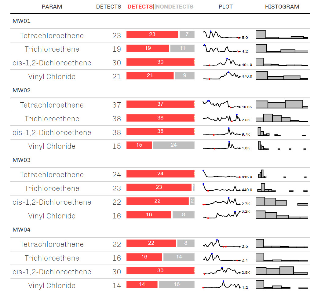
We can use the R package gtExtras to create a sparkline table of the concentration data. A sparkline is a very small line chart, typically drawn without axes or coordinates. It presents the general shape of the measurement variation (typically over time) in a simple and highly condensed way. Sparklines can be used to help identify patterns in the data, such as trends or temporal variability. The results are shown below for four of the 31 wells. I’ve included the number of detects and non-detects, a time-series line plot, and a histogram fro each well and parameter.
# View graphical summary of concentration data
library(gt)
library(gtExtras)

bb <- dat %>%
  dplyr::group_by(LOCID, PARAM) %>%
  dplyr::summarize(
    Plot = list(RESULT2),
    Histogram = list(RESULT2),
    .groups = "drop"
  ) %>%
  ungroup()

zz <- dat %>%
  group_by(LOCID, PARAM) %>%
  summarize(
    DET = length(RESULT2[DETECTED == 'Y']),
    ND = length(RESULT2[DETECTED == 'N'])
  ) %>%
  ungroup() %>%
  tidyr::gather(condition, count, DET:ND) %>%
  arrange(LOCID, PARAM, condition) %>%
  group_by(LOCID, PARAM) %>%
  summarize(detects = count[1], list_data = list(count))

zz %>%
  left_join(bb, by = c('LOCID', 'PARAM')) %>%
  filter(LOCID %in% c('MW01', 'MW02', 'MW03', 'MW04')) %>%
  gt() %>%
  gt_plt_bar_stack(
    list_data, width = 40,
    labels = c("Detects", "Nondetects"),
    palette= c("#ff4343", "#bfbfbf")
  ) %>%
  gt_sparkline(Plot, same_limit = FALSE) %>%
  gt_sparkline(Histogram, type = 'histogram', same_limit = FALSE) %>%
  gt_theme_538()
Duplicates
A fundamental assumption governing almost every statistical procedure and test is the presumption that sample data from a given population should be independent and identically distributed. If this assumption is not satisfied, statistical conclusions and test results may be invalid or in error (USEPA 2009). Measurements from a truly random sampling of a population will be statistically independent. This means that observing or knowing the value of one measurement does not alter or influence the probability of observing any other measurement in the population. Duplicate sample results are generally not independent; significant positive correlation almost always exists between duplicate samples.
Although duplicate sample results can provide valuable information about the level of measurement variability attributable to sampling or analytical techniques, they should not be treated as separate observations in statistical calcuations. One strategy is to simply average each set of duplicate results and treat the resulting mean as a single observation in the overall data set. Despite eliminating the dependence between the duplicates, such averaging is not an ideal solution. The variability in means of two correlated measurements is approximately 30% less than the variability associated with two single independent measurements (USEPA 2009). If a data set consists of a mixture of single measurements and duplicates, the variability of the averaged values will be less than the variability of the single measurements. This would imply that the final data set is not identically distributed.
It is important to remove duplicate results from the data before calculating summary statistics, such as the mean and variance, because these statistics assume independent data. Let’s check our data for duplicate samples based on well name (LOCID), sample date (LOGDATE), and parameter name (PARAM).
# Check for dulicates
xx <- dat[duplicated(dat[c('LOCID', 'LOGDATE', 'PARAM')]),]
if (length(xx$LOCID) > 0) {
    print('Duplicates found in the input data. The duplicates are shown below:')
    xx
} else {
    print('No duplicates found in the input data.')
}
## [1] "No duplicates found in the input data."
Statistics
Now that we have prepped and examined the data, let’s calculate some statistics using the trendMK package. Most functions in trendMK use the same general input format, although some functions may have additional input requirements. The general input requirements consist of the following:
- x = vector of date-ordered measurements
- detect = vector of logical values indicating whether measurements are detects (“Y”) or non-detects (“N”)
- date = vector of calendar dates when measurements were made (format must be m/d/yyyy)
- loc = vector of location ids where measurements were taken
- param = vector of parameter names
- censor_limit = character name of variable containing the censoring limit (e.g., MDL, LOD, RL) used for non-detects
- units_field = character name of variable containing the units of measurement
- flag_field = character name of variable containing the data qualifiers, where NA can be used if no qualifiers are present in the data
The easiest way to run a trendMK function is using the with() function. The with() function applys an expression to a dataset and is a wrapper for functions with no data argument. This is shown in the many examples provide below.
The help() function and ? help operator in R provides access to the documentation pages for R functions, data sets, and other objects, both for packages in the standard R distribution and for contributed packages. To access documentation for the sumstats() function in trendMK, for example, enter the command help(sumstats) or ?sumstats.
Summary Statistics
Let’s calculate summary statistics for all four of the VOCs in each individual monitoring well. The output is a data frame that includes the total number of samples, the number of detected and non-detected observations, and the frequency of detection; the minimum and maximum values for detected and non-detected observations; and the mean, median, standard deviation, and coefficient of variation (CV); and the last sample result and samplpe date. The mean and median provide a measure of central tendency, while the standard deviation and CV provide a measure of variability in the data. The CV is the ratio of the sample standard deviation to the sample mean and thus indicates whether the amount of “spread” in the data is small or large relative to the average observed magnitude. Values less than one indicate that the standard deviation is smaller than the mean, while values greater than one occur when the standard deviation is greater than the mean.
The Kaplan-Meier (KM) product-limit estimator (Kaplan and Meier 1958) is used to estimate the mean, median, and standard deviation for data sets containing non-detects. In the KM method, a percentile is assigned to each detected observation, starting at the largest detected value and working down the data set, based on the number of detects and non-detects above and below each observation. Percentiles are not assigned to non-detects, but non-detects affect the percentiles calculated for detected observations. The survival curve, a step function plot of the cumulative distribution function, gives the shape of the data set. Estimates of the mean and standard deviation are computed from the estimated cumulative distribution function and these estimates then can be used in parametric statistical tests.
The USEPA (2015) recommend the use of the KM method for data sets containing non-detects with multiple detection or reporting limits. Although substitution of one-half the censoring limit (MDL, LOD, RL) for non-detects has been incorporated in the code and can be selected by the user via the method variable, its use is not recommended due to its poor performance. The substitution method has been retained for historical and comparison purposes.
Summary statistics are not calculated when the detection frequency is less than 50%. If a data set is a mixture of detects and non-detects, but the non-detect fraction is no more than 50%, a censored estimation method such as the KM method can be used to compute adjusted estimates of the mean and standard deviation. Because parameter estimation can suffer for data sets with low detection frequencies, the EPA (2009) recommends that these methods should not be used when more than 50% of the data are non-detects.
The summary statistics calculated using the sumstats() function can be saved as a csv file to our working directory using R’s write.table() function with the separator variable set to a comma (sep = “,”). The code is shown below.
# Get summary statistics
sum_stats <- with(dat,
  sumstats(
    x = RESULT,
    detect = DETECTED,
    date = LOGDATE,
    loc = LOCID,
    param = PARAM,
    censor_limit = MDL,
    units_field = UNITS,
    flag_field = QUALIFIERS,
    method = 'KM'
  )
)
sum_stats
## # A tibble: 124 x 17
##    PARAM   LOCID UNITS COUNT   DET   CEN PER.DET MIN.CEN MAX.CEN MIN.DET MAX.DET
##    <ord>   <chr> <chr> <int> <int> <int>   <dbl>   <dbl>   <dbl>   <dbl>   <dbl>
##  1 Tetrac~ MW01  µg/L     30    23     7    76.7     0.5    10     17       1850
##  2 Tetrac~ MW02  µg/L     37    37     0   100      NA      NA   1210     150000
##  3 Tetrac~ MW03  µg/L     24    24     0   100      NA      NA    816     239000
##  4 Tetrac~ MW04  µg/L     30    22     8    73.3     2.8    62      3.28    4240
##  5 Tetrac~ MW05  µg/L     28    28     0   100      NA      NA    226      19500
##  6 Tetrac~ MW06  µg/L     28    26     2    92.9    14      24.8   19.4    10600
##  7 Tetrac~ MW07  µg/L     28    28     0   100      NA      NA    177     104000
##  8 Tetrac~ MW08  µg/L     24    22     2    91.7     6.2    14      2.9    28200
##  9 Tetrac~ MW09  µg/L     38    38     0   100      NA      NA    371     350000
## 10 Tetrac~ MW10  µg/L     39    39     0   100      NA      NA    121      34000
## # ... with 114 more rows, and 6 more variables: MEAN <dbl>, MEDIAN <dbl>,
## #   SD <dbl>, CV <dbl>, LASTVALUE <chr>, LASTDATE <date>
# Not run
# Save results to csv file
#outfile <- 'sumstats.csv'
#write.table(sum_stats, file = outfile, sep = ",",
#  row.names = F, col.names = T, append = F)
Mann-Kendall Test
The Mann-Kendall test (Mann 1945; Kendall 1975; Gilbert 1987) is a nonparametric procedure used to assess if there is a monotonic upward or downward trend of the variable of interest over time. A monotonic upward (downward) trend means that the variable consistently increases (decreases) through time, but the trend may or may not be linear. The data values are evaluated as an ordered time series where each data value is compared to all subsequent data values. Thus, the test can be viewed as a nonparametric test for zero slope of the linear regression of time-ordered data versus time, as illustrated by Hollander and Wolfe (1973, p. 201). Non-detects can be included in the test by assigning them a common value that is less than the smallest measured value in the data set (USEPA 2009).
The Mann-Kendall test statistic (S) is found by counting the number of “concordant observations”, where the later-in-time observation has a larger value for the series, and subtracting the number of “discordant observations”, where the later-in-time observation has a smaller value for the series. This is done for all pairs of observations in the data set. The total difference is denoted S. Positive values of S indicate an increase in constituent concentrations over time, whereas negative values indicate a decrease in constituent concentrations over time. The strength of the trend is proportional to the magnitude of S (i.e., the larger the absolute value of S, the stronger the evidence for a real increasing or decreasing trend).
The null hypothesis in the Mann-Kendall test assumes that there is no trend (the data are independent and randomly ordered) and this is tested against the alternative hypothesis, which assumes that there is a trend. The calculated probability (p-value) of the test represents the probability that any observed trend would occur purely by chance (given the variability and sample size of the data set). A significance level of 0.05 (i.e., 95% confidence) typically is used to test the null hypothesis that there is no trend in the data. The significance level is the probability that a test erroneously detects a trend when none is present. Only p-values less than the significance level indicate a statistically significant trend.
For wells exhibiting a statistically significant trend in constituent concentrations, the slope in the data is estimated using the method of Theil (1950) and Sen (1968) to gauge the magnitude of the trend. Although nonparametric, the Theil-Sen slope estimator does not use data ranks but rather the concentrations themselves. The method is nonparametric because the median pairwise slope is utilized, thus ignoring extreme values that might otherwise skew the slope estimate. Consequently, the Theil-Sen line estimates the change in median concentration over time and not the mean as in linear regression. The Theil-Sen method handles non-detects in the same manner as the Mann-Kendall test; it assigns each non-detect a common value less than any detected measurement (USEPA 2009). Unlike the Mann-Kendall test, however, the actual concentration values are important in computing the slope estimate in the Theil-Sen procedure. Therefore, the approach is not appropriate when more than 50% of the concentration measurements are non-detects (ITRC 2013).
Let’s perform trend analysis at a significance level of 0.05 (95% confidence) for all four VOCs in each individual monitoring well using the trend() function. The results are shown below. These results can be saved as a csv file to our working directory using R’s write.table() function with the separator variable set to a comma (sep = “,”). The code is shown below.
# Get Mann-Kendall trend trends
trends <- with(dat,
  trend(
    x = RESULT,
    detect = DETECTED,
    date = LOGDATE,
    loc = LOCID,
    param = PARAM,
    censor_limit = MDL,
    units_field = UNITS,
    flag_field = QUALIFIERS,
    method = 'KM',
    alpha = 0.05
  )
)

# Inspect output
str(trends)
## 'data.frame':	124 obs. of  24 variables:
##  $ LOCID    : chr  "MW01" "MW02" "MW03" "MW04" ...
##  $ PARAM    : Ord.factor w/ 4 levels "Tetrachloroethene"<..: 1 1 1 1 1 1 1 1 1 1 ...
##  $ UNITS    : chr  "µg/L" "µg/L" "µg/L" "µg/L" ...
##  $ COUNT    : int  30 37 24 30 28 28 28 24 38 39 ...
##  $ DET      : int  23 37 24 22 28 26 28 22 38 39 ...
##  $ CEN      : int  7 0 0 8 0 2 0 2 0 0 ...
##  $ PER.DET  : num  76.7 100 100 73.3 100 ...
##  $ MIN.CEN  : num  0.5 NA NA 2.8 NA 14 NA 6.2 NA NA ...
##  $ MAX.CEN  : num  10 NA NA 62 NA 24.8 NA 14 NA NA ...
##  $ MIN.DET  : num  17 1210 816 3.28 226 19.4 177 2.9 371 121 ...
##  $ MAX.DET  : num  1850 150000 239000 4240 19500 10600 104000 28200 350000 34000 ...
##  $ MEAN     : num  476 69159 27284 775 7113 ...
##  $ MEDIAN   : num  100.1 73100 12500 89.4 3900 ...
##  $ SD       : num  660 49850 52347 1200 6789 ...
##  $ CV       : num  1.386 0.721 1.919 1.55 0.954 ...
##  $ LASTVALUE: chr  "10 U" "10600 " "816 " "5 U" ...
##  $ LASTDATE : Date, format: "2021-04-14" "2021-04-16" ...
##  $ S        : chr  "-284" "-289" "-87" "-215" ...
##  $ PVAL     : chr  "1.83795918928809e-07" "8.25972529128194e-05" "0.016" "5.70869560760912e-05" ...
##  $ SLOPE    : num  -46.6 -7632.3 -1728.1 -38.2 -469.4 ...
##  $ RESULT   : chr  "100% (sig -)" "100% (sig -)" "98.4% (sig -)" "100% (sig -)" ...
##  $ TREND    : chr  "Decreasing" "Decreasing" "Decreasing" "Decreasing" ...
##  $ STABILITY: chr  NA NA NA NA ...
##  $ MIN.LAG  : num  37 38 30 34 37 39 30 65 35 34 ...
head(trends)
##    LOCID             PARAM UNITS COUNT DET CEN PER.DET MIN.CEN MAX.CEN MIN.DET
## 32  MW01 Tetrachloroethene  µg/L    30  23   7   76.67     0.5    10.0   17.00
## 33  MW02 Tetrachloroethene  µg/L    37  37   0  100.00      NA      NA 1210.00
## 34  MW03 Tetrachloroethene  µg/L    24  24   0  100.00      NA      NA  816.00
## 35  MW04 Tetrachloroethene  µg/L    30  22   8   73.33     2.8    62.0    3.28
## 36  MW05 Tetrachloroethene  µg/L    28  28   0  100.00      NA      NA  226.00
## 37  MW06 Tetrachloroethene  µg/L    28  26   2   92.86    14.0    24.8   19.40
##    MAX.DET       MEAN  MEDIAN        SD        CV LASTVALUE   LASTDATE    S
## 32    1850   475.8533   100.1   659.522 1.3859776      10 U 2021-04-14 -284
## 33  150000 69158.9189 73100.0 49849.989 0.7208035    10600  2021-04-16 -289
## 34  239000 27284.0000 12500.0 52347.302 1.9186081      816  2021-04-15  -87
## 35    4240   774.6624    89.4  1200.379 1.5495513       5 U 2021-04-14 -215
## 36   19500  7113.2857  3900.0  6789.396 0.9544669      972  2021-04-14 -126
## 37   10600  3761.4321  2180.0  3509.968 0.9331466    19.4 J 2021-04-16 -210
##                    PVAL       SLOPE        RESULT      TREND STABILITY MIN.LAG
## 32 1.83795918928809e-07   -46.55213  100% (sig -) Decreasing      <NA>      37
## 33 8.25972529128194e-05 -7632.32215  100% (sig -) Decreasing      <NA>      38
## 34                0.016 -1728.05554 98.4% (sig -) Decreasing      <NA>      30
## 35 5.70869560760912e-05   -38.15017  100% (sig -) Decreasing      <NA>      34
## 36                0.006  -469.35370 99.4% (sig -) Decreasing      <NA>      37
## 37 1.80810475285398e-05  -546.89507  100% (sig -) Decreasing      <NA>      39
# Not run
# Save results to csv file
#outfile <- 'trend_summary.csv'
#write.table(trends, file = outfile, sep = ",",
#  row.names = F, col.names = T, append = F)
Note that in the output where there is insufficient evidence for identifying a significant, non-zero trend, concentrations are deemed stable if the CV is less than 1. The CV is recognized as an acceptable measure of intrinsic variability in positive-valued data sets (USEPA 2009) and can be used as an indication of stability. Values less than or near 1 indicate that the data form a relatively close group about the mean value. Values larger than 1 indicate that the data show a greater degree of scatter about the mean. It should be noted that the CV is a relative measure of variation in groundwater concentration data and can be affected by the magnitude of concentration (USEPA 2009). As such, relatively higher concentrations can include significant variation while exhibiting a small CV.
The output includes a column named MIN.LAG, which represents the minimum sampling spacing for each well and constituent. An underlying assumption in the Mann-Kendall test (Mann 1945; Kendall 1975; Gilbert 1987) is that the data are not serially correlated. Successive measurements in time series from groundwater monitoring are often correlated with one another, especially when the groundwater is slow-moving, and wells are being sampled on closely-spaced sampling events. This means that pairs of consecutive measurements taken in a series will be positively correlated, exhibiting a stronger similarity in concentration levels than expected from pairs collected at random times. A positive serial correlation increases the likelihood of rejecting the null hypothesis of no trend when it might be true (the probability of the Type 1 error becomes larger than what the attained significance level indicates).
Let’s see if any of the trend results are associated with data containing a minimum spacing between consecutive samples that is less than or equal to 30 days. Below, we see that the minimum spacing between consecutive samples is 30 days and occurs for nine constitutent/well pairs.
# Inspect results where minimum spacing between consecutive sample results is
# less than or equal to 30 days
trends[trends$MIN.LAG <= 30, ]
##     LOCID                  PARAM UNITS COUNT DET CEN PER.DET MIN.CEN MAX.CEN
## 34   MW03      Tetrachloroethene  µg/L    24  24   0  100.00      NA      NA
## 38   MW07      Tetrachloroethene  µg/L    28  28   0  100.00      NA      NA
## 65   MW03        Trichloroethene  µg/L    24  23   1   95.83    22.4    22.4
## 69   MW07        Trichloroethene  µg/L    28  19   9   67.86    44.9   790.0
## 3    MW03 cis-1,2-Dichloroethene  µg/L    24  22   2   91.67   735.0   735.0
## 7    MW07 cis-1,2-Dichloroethene  µg/L    28  19   9   67.86    36.7   367.0
## 96   MW03         Vinyl Chloride  µg/L    24  16   8   66.67    20.1   804.0
## 99   MW06         Vinyl Chloride  µg/L    29  27   2   93.10    80.4    80.4
## 100  MW07         Vinyl Chloride  µg/L    28  13  15   46.43    18.0   402.0
##     MIN.DET MAX.DET       MEAN  MEDIAN         SD        CV LASTVALUE
## 34    816.0  239000 27284.0000 12500.0 52347.3020 1.9186081      816
## 38    177.0  104000 17789.9286 11250.0 22035.6665 1.2386596      177
## 65    174.0    4880   839.4750   469.5  1086.9858 1.2948400     440 J
## 69     62.2   12200   751.5396   224.0  2236.0289 2.9752642      121
## 3     522.0   68500 18304.6667 16100.0 17945.6914 0.9803889     2670
## 7      44.6  106000 25896.9964   380.5 34022.3443 1.3137564   106000
## 96    149.0    3250   996.6617   871.0   978.3699 0.9816470     3180
## 99     10.9   27800  8304.4034  3650.0  9028.5789 1.0872038    14100
## 100    30.6    8100         NA      NA         NA        NA     4860
##       LASTDATE    S                 PVAL      SLOPE        RESULT      TREND
## 34  2021-04-15  -87                0.016 -1728.0555 98.4% (sig -) Decreasing
## 38  2021-04-17 -262 1.25836635334053e-07 -2566.7495  100% (sig -) Decreasing
## 65  2021-04-15  -16                0.356         NA     64.4% (-)   No Trend
## 69  2021-04-17   82                0.055         NA     94.5% (+)   No Trend
## 3   2021-04-15   69                0.046  1685.4768 95.4% (sig +) Increasing
## 7   2021-04-17  290                    0  4758.6402  100% (sig +) Increasing
## 96  2021-04-15  149 8.89897346496582e-05   153.0901  100% (sig +) Increasing
## 99  2021-04-16  184 0.000297427177429199  1125.6479  100% (sig +) Increasing
## 100 2021-04-17  189 2.55107879638672e-05   298.7621  100% (sig +) Increasing
##      STABILITY MIN.LAG
## 34        <NA>      30
## 38        <NA>      30
## 65  Not Stable      30
## 69  Not Stable      30
## 3         <NA>      30
## 7         <NA>      30
## 96        <NA>      30
## 99        <NA>      30
## 100       <NA>      30
Let’s quickly get a summary of the trend analysis results. We see that of the 124 cases (constituent/well pairs) evaluated with the Mann-Kendall test, there are 107 cases with a statistically significant trend at the 95% confidence level. There are 55 increasing trends and 52 decreasing trends.
# Get number of statistically significant trends
all_trend <- length(trends$TREND)
inc_trend <- length(trends[trends$TREND == 'Increasing', ]$TREND)
dec_trend <- length(trends[trends$TREND == 'Decreasing', ]$TREND)

trend_counts <- paste(
  'The total cases evaluated with the Mann-Kendall test is', all_trend,
  ' \nThe total number of statistically significant trends is', inc_trend + dec_trend,
  ' \nThe number of increasing trends is', inc_trend,
  ' \nThe number of decreasing trends is', dec_trend
)

cat(trend_counts)
## The total cases evaluated with the Mann-Kendall test is 124
## The total number of statistically significant trends is 107
## The number of increasing trends is 55
## The number of decreasing trends is 52
Let’s inspect the constituents and wells that have an increasing trend.
# Inspect results where trends are increasing
trends[trends$TREND == 'Increasing', ]
##     LOCID                  PARAM UNITS COUNT DET CEN PER.DET MIN.CEN MAX.CEN
## 71   MW09        Trichloroethene  µg/L    39  27  12   69.23 224.000  4500.0
## 75   MW13        Trichloroethene  µg/L    36  36   0  100.00      NA      NA
## 81   MW19        Trichloroethene  µg/L    32  31   1   96.88 395.000   395.0
## 82   MW20        Trichloroethene  µg/L    28  28   0  100.00      NA      NA
## 1    MW01 cis-1,2-Dichloroethene  µg/L    30  30   0  100.00      NA      NA
## 2    MW02 cis-1,2-Dichloroethene  µg/L    38  38   0  100.00      NA      NA
## 3    MW03 cis-1,2-Dichloroethene  µg/L    24  22   2   91.67 735.000   735.0
## 4    MW04 cis-1,2-Dichloroethene  µg/L    30  30   0  100.00      NA      NA
## 5    MW05 cis-1,2-Dichloroethene  µg/L    28  28   0  100.00      NA      NA
## 7    MW07 cis-1,2-Dichloroethene  µg/L    28  19   9   67.86  36.700   367.0
## 9    MW09 cis-1,2-Dichloroethene  µg/L    39  22  17   56.41 184.000  3700.0
## 10   MW10 cis-1,2-Dichloroethene  µg/L    39  39   0  100.00      NA      NA
## 11   MW11 cis-1,2-Dichloroethene  µg/L    37  37   0  100.00      NA      NA
## 13   MW13 cis-1,2-Dichloroethene  µg/L    37  33   4   89.19 184.000   920.0
## 15   MW15 cis-1,2-Dichloroethene  µg/L    32  32   0  100.00      NA      NA
## 16   MW16 cis-1,2-Dichloroethene  µg/L    34  34   0  100.00      NA      NA
## 17   MW17 cis-1,2-Dichloroethene  µg/L    33  33   0  100.00      NA      NA
## 18   MW18 cis-1,2-Dichloroethene  µg/L    32  32   0  100.00      NA      NA
## 19   MW19 cis-1,2-Dichloroethene  µg/L    32  31   1   96.88  36.700    36.7
## 20   MW20 cis-1,2-Dichloroethene  µg/L    28  28   0  100.00      NA      NA
## 21   MW21 cis-1,2-Dichloroethene  µg/L    28  21   7   75.00 184.000   735.0
## 23   MW23 cis-1,2-Dichloroethene  µg/L    28  28   0  100.00      NA      NA
## 24   MW24 cis-1,2-Dichloroethene  µg/L    27  27   0  100.00      NA      NA
## 27   MW27 cis-1,2-Dichloroethene  µg/L    27  26   1   96.30  18.400    18.4
## 28   MW28 cis-1,2-Dichloroethene  µg/L    24  22   2   91.67  11.700   367.0
## 29   MW29 cis-1,2-Dichloroethene  µg/L    24  18   6   75.00  18.400    18.4
## 94   MW01         Vinyl Chloride  µg/L    30  21   9   70.00   0.402    26.9
## 95   MW02         Vinyl Chloride  µg/L    39  15  24   38.46  40.200  2000.0
## 96   MW03         Vinyl Chloride  µg/L    24  16   8   66.67  20.100   804.0
## 97   MW04         Vinyl Chloride  µg/L    30  14  16   46.67   1.000   107.0
## 98   MW05         Vinyl Chloride  µg/L    28  23   5   82.14  20.100   201.0
## 99   MW06         Vinyl Chloride  µg/L    29  27   2   93.10  80.400    80.4
## 100  MW07         Vinyl Chloride  µg/L    28  13  15   46.43  18.000   402.0
## 101  MW08         Vinyl Chloride  µg/L    24  15   9   62.50  40.200   537.0
## 102  MW09         Vinyl Chloride  µg/L    39   9  30   23.08   9.000  4000.0
## 103  MW10         Vinyl Chloride  µg/L    40  19  21   47.50  10.000   400.0
## 104  MW11         Vinyl Chloride  µg/L    38  17  21   44.74  80.400   537.0
## 105  MW12         Vinyl Chloride  µg/L    27  15  12   55.56  80.400  1000.0
## 106  MW13         Vinyl Chloride  µg/L    37  12  25   32.43  90.000  1070.0
## 107  MW14         Vinyl Chloride  µg/L    36  11  25   30.56   0.180    26.9
## 108  MW15         Vinyl Chloride  µg/L    34  18  16   52.94  20.100   537.0
## 109  MW16         Vinyl Chloride  µg/L    35  18  17   51.43  20.100   400.0
## 110  MW17         Vinyl Chloride  µg/L    34  26   8   76.47   0.402   800.0
## 111  MW18         Vinyl Chloride  µg/L    33  17  16   51.52  80.000   537.0
## 112  MW19         Vinyl Chloride  µg/L    34  17  17   50.00   1.070   201.0
## 113  MW20         Vinyl Chloride  µg/L    29  19  10   65.52   8.040    80.4
## 114  MW21         Vinyl Chloride  µg/L    28   4  24   14.29   3.600   804.0
## 115  MW22         Vinyl Chloride  µg/L    28  16  12   57.14   2.010    80.4
## 116  MW23         Vinyl Chloride  µg/L    29  16  13   55.17  18.000   402.0
## 117  MW24         Vinyl Chloride  µg/L    28  14  14   50.00   1.800    40.2
## 119  MW26         Vinyl Chloride  µg/L    28   6  22   21.43   0.900    40.2
## 120  MW27         Vinyl Chloride  µg/L    28   9  19   32.14   0.900    40.2
## 121  MW28         Vinyl Chloride  µg/L    24   6  18   25.00   1.800   402.0
## 122  MW29         Vinyl Chloride  µg/L    24  10  14   41.67   0.180    32.6
## 123  MW30         Vinyl Chloride  µg/L    23  16   7   69.57 201.000   804.0
##     MIN.DET  MAX.DET       MEAN  MEDIAN         SD        CV LASTVALUE
## 71  234.000   7300.0  1533.6594  1100.0  1713.5188 1.1172747      244
## 75  669.000  23400.0  4673.0278  2050.0  6056.2274 1.2959965    1290 J
## 81    3.610   5110.0   940.7562   432.5  1219.6883 1.2964978     1310
## 82  144.000   4070.0  1387.6786   746.5  1303.8004 0.9395550     2410
## 1    11.900  13300.0  3042.4933   723.5  4094.2140 1.3456772      494
## 2   391.000 166000.0 17779.7105  5775.0 30456.7326 1.7130050     9720
## 3   522.000  68500.0 18304.6667 16100.0 17945.6914 0.9803889     2670
## 4    90.200  15500.0  5433.7567  3440.0  4544.0778 0.8362682     2780
## 5   719.000  67000.0 13598.2143  6405.0 18196.3635 1.3381436     7240
## 7    44.600 106000.0 25896.9964   380.5 34022.3443 1.3137564   106000
## 9   140.000  44500.0  5081.8258   920.0  8483.0305 1.6692879     2470
## 10   64.300  48600.0  8149.3410  1800.0 10902.9874 1.3378980    13600
## 11    0.780  81200.0 21043.2373  7060.0 23797.5374 1.1308877    44500
## 13  204.000  39300.0  6848.0865  1070.0 10103.6213 1.4753934     4090
## 15  399.000  44800.0 13191.0625 10135.0 13454.5818 1.0199771     5900
## 16  208.000  26300.0  6880.1176   897.5  8772.1294 1.2749970     1200
## 17   13.600  81300.0 25070.4121 15200.0 21717.5045 0.8662604    33700
## 18  170.000  24700.0  6950.9062  5385.0  6386.0989 0.9187434     3390
## 19   42.200  57200.0  9662.6875  1980.0 12737.3094 1.3181953    19700
## 20  128.000  31800.0  8427.9286  3395.0 10002.7292 1.1868550    13300
## 21  111.000   1550.0   435.2627   371.0   338.5217 0.7777411      483
## 23  351.000  18200.0  5614.9286  5260.0  5228.9113 0.9312516     6970
## 24   10.500   4090.0   919.2444   740.0  1038.3116 1.1295271      281
## 27  137.000    928.0   411.3481   380.0   194.6655 0.4732378      202
## 28  104.000  11700.0  4090.1406  4245.0  2997.5040 0.7328609     1530
## 29   10.300   1220.0   174.8167    55.2   297.7584 1.7032610     74.1
## 94   16.500   1360.0   416.8483   319.5   450.5063 1.0807439      470
## 95  687.000  24900.0         NA      NA         NA        NA     1560
## 96  149.000   3250.0   996.6617   871.0   978.3699 0.9816470     3180
## 97   49.400    749.0         NA      NA         NA        NA    2.34 U
## 98   85.200   2720.0   727.6510   292.0   815.3690 1.1205496      449
## 99   10.900  27800.0  8304.4034  3650.0  9028.5789 1.0872038    14100
## 100  30.600   8100.0         NA      NA         NA        NA     4860
## 101   3.320   5630.0   453.5848    93.6  1172.4705 2.5848980     61.1
## 102  10.300    309.0         NA      NA         NA        NA      188
## 103  14.100   5950.0         NA      NA         NA        NA     1380
## 104 130.000  26800.0         NA      NA         NA        NA    10600
## 105  21.400   3340.0   534.9215   650.0   801.2822 1.4979437     46.6
## 106 107.000   9160.0         NA      NA         NA        NA      110
## 107   0.599    205.0         NA      NA         NA        NA    1.91 J
## 108 368.000   9710.0  1754.0695   553.5  2624.6055 1.4962950     1910
## 109   8.940   5130.0  1151.6866   205.0  1457.2497 1.2653179      738
## 110 181.000  17400.0  4028.0347   800.0  5172.3791 1.2840950     9200
## 111 109.000   1090.0   299.8723   381.0   234.6138 0.7823789      191
## 112 318.000  24500.0  2135.5056   259.5  4300.0078 2.0135783     2720
## 113   3.590   6010.0  1226.6684   262.0  1699.3496 1.3853374     2600
## 114   0.770     15.4         NA      NA         NA        NA     15.4
## 115  22.500   1300.0   283.0780   139.5   372.1704 1.3147277      548
## 116 336.000   2490.0   798.7056   566.0   847.1719 1.0606811     979 J
## 117   4.790    824.0   153.1934    20.1   226.9723 1.4816068     78.9
## 119   0.621    168.0         NA      NA         NA        NA     69.5
## 120   1.150    108.0         NA      NA         NA        NA      103
## 121   6.760     71.9         NA      NA         NA        NA     25.6
## 122   5.710     46.7         NA      NA         NA        NA     31.3
## 123 766.000   3890.0  1511.5528  1680.0  1075.8937 0.7117804     1100
##       LASTDATE   S                 PVAL       SLOPE        RESULT      TREND
## 71  2021-04-14 453                    0  216.964156  100% (sig +) Increasing
## 75  2021-04-16 159   0.0156553983688354  163.411811 98.4% (sig +) Increasing
## 81  2021-04-15 165  0.00390070676803589  107.062545 99.6% (sig +) Increasing
## 82  2021-04-15 252 3.57627868652344e-07  253.436018  100% (sig +) Increasing
## 1   2021-04-14 169  0.00136196613311768  282.346765 99.9% (sig +) Increasing
## 2   2021-04-16 319  3.1888484954834e-05 1325.196238  100% (sig +) Increasing
## 3   2021-04-15  69                0.046 1685.476815 95.4% (sig +) Increasing
## 4   2021-04-14 179 0.000747382640838623  747.907648 99.9% (sig +) Increasing
## 5   2021-04-14 198 4.97102737426758e-05 1313.580623  100% (sig +) Increasing
## 7   2021-04-17 290                    0 4758.640184  100% (sig +) Increasing
## 9   2021-04-14 457                    0  603.994072  100% (sig +) Increasing
## 10  2021-04-14 386 1.60932540893555e-06 1084.830762  100% (sig +) Increasing
## 11  2021-04-15 341 4.35113906860352e-06 3029.717084  100% (sig +) Increasing
## 13  2021-04-16 390 1.78813934326172e-07  938.296672  100% (sig +) Increasing
## 15  2021-04-16 267 7.98702239990234e-06 1541.025970  100% (sig +) Increasing
## 16  2021-04-16 338 2.98023223876953e-07 1286.792839  100% (sig +) Increasing
## 17  2021-04-16 264 2.30073928833008e-05 3261.966584  100% (sig +) Increasing
## 18  2021-04-15 268 7.45058059692383e-06  981.435865  100% (sig +) Increasing
## 19  2021-04-15 304 4.76837158203125e-07 1799.678666  100% (sig +) Increasing
## 20  2021-04-15 285                    0 1527.028649  100% (sig +) Increasing
## 21  2021-04-13 183 0.000143229961395264   45.221971  100% (sig +) Increasing
## 23  2021-04-15 165 0.000596165657043457  735.866381 99.9% (sig +) Increasing
## 24  2021-04-14 142                0.001  114.274840 99.9% (sig +) Increasing
## 27  2021-04-14 133                0.003   26.243983 99.7% (sig +) Increasing
## 28  2021-04-13  76                0.031  385.749042 96.9% (sig +) Increasing
## 29  2021-04-13 121                0.001   11.713974 99.9% (sig +) Increasing
## 94  2021-04-14 179 0.000633716583251953   70.069644 99.9% (sig +) Increasing
## 95  2021-04-16 336 1.72853469848633e-06   69.105261  100% (sig +) Increasing
## 96  2021-04-15 149 8.89897346496582e-05  153.090113  100% (sig +) Increasing
## 97  2021-04-14 199  5.9664249420166e-05   14.851330  100% (sig +) Increasing
## 98  2021-04-14 192  7.6591968536377e-05  101.182321  100% (sig +) Increasing
## 99  2021-04-16 184 0.000297427177429199 1125.647915  100% (sig +) Increasing
## 100 2021-04-17 189 2.55107879638672e-05  298.762081  100% (sig +) Increasing
## 101 2021-04-16  96                0.009    2.986496 99.1% (sig +) Increasing
## 102 2021-04-14 262                0.001    0.000000 99.9% (sig +) Increasing
## 103 2021-04-14 358 3.27825546264648e-06   84.380469  100% (sig +) Increasing
## 104 2021-04-15 302 1.57356262207031e-05  823.764257  100% (sig +) Increasing
## 105 2021-04-15 109                0.012    2.611858 98.8% (sig +) Increasing
## 106 2021-04-16 248                    0    0.000000  100% (sig +) Increasing
## 107 2021-04-16 256  9.5367431640625e-06    0.000000  100% (sig +) Increasing
## 108 2021-04-16 369                    0  199.710216  100% (sig +) Increasing
## 109 2021-04-16 284 9.23871994018555e-06  162.744676  100% (sig +) Increasing
## 110 2021-04-16 313 1.60932540893555e-06  701.828584  100% (sig +) Increasing
## 111 2021-04-15 212 0.000248849391937256   25.083209  100% (sig +) Increasing
## 112 2021-04-15 255 2.71797180175781e-05  204.486907  100% (sig +) Increasing
## 113 2021-04-15 301                    0  205.931452  100% (sig +) Increasing
## 114 2021-04-13  94                0.033    0.000000 96.7% (sig +) Increasing
## 115 2021-04-14 166   0.0003318190574646   24.812957  100% (sig +) Increasing
## 116 2021-04-15 222 6.61611557006836e-06  133.736704  100% (sig +) Increasing
## 117 2021-04-14 179 8.13603401184082e-05   10.312136  100% (sig +) Increasing
## 119 2021-04-14 131               0.0045    0.000000 99.6% (sig +) Increasing
## 120 2021-04-14 167 3.53455543518066e-05    0.000000  100% (sig +) Increasing
## 121 2021-04-13  93               0.0105    0.000000   99% (sig +) Increasing
## 122 2021-04-13 135 9.63211059570312e-05    2.536911  100% (sig +) Increasing
## 123 2021-04-15  95                0.006  190.459982 99.4% (sig +) Increasing
##     STABILITY MIN.LAG
## 71       <NA>      35
## 75       <NA>      34
## 81       <NA>      37
## 82       <NA>      65
## 1        <NA>      34
## 2        <NA>      35
## 3        <NA>      30
## 4        <NA>      34
## 5        <NA>      37
## 7        <NA>      30
## 9        <NA>      34
## 10       <NA>      34
## 11       <NA>      38
## 13       <NA>      34
## 15       <NA>      37
## 16       <NA>      35
## 17       <NA>      39
## 18       <NA>      34
## 19       <NA>      37
## 20       <NA>      65
## 21       <NA>      36
## 23       <NA>      61
## 24       <NA>      61
## 27       <NA>      63
## 28       <NA>      62
## 29       <NA>      63
## 94       <NA>      35
## 95       <NA>      33
## 96       <NA>      30
## 97       <NA>      33
## 98       <NA>      37
## 99       <NA>      30
## 100      <NA>      30
## 101      <NA>      65
## 102      <NA>      34
## 103      <NA>      34
## 104      <NA>      33
## 105      <NA>      36
## 106      <NA>      34
## 107      <NA>      35
## 108      <NA>      34
## 109      <NA>      34
## 110      <NA>      35
## 111      <NA>      34
## 112      <NA>      33
## 113      <NA>      35
## 114      <NA>      36
## 115      <NA>      35
## 116      <NA>      35
## 117      <NA>      35
## 119      <NA>      35
## 120      <NA>      35
## 121      <NA>      62
## 122      <NA>      63
## 123      <NA>      64
Let’s create a summary table by spreading the trend results. After spreading the results, we can save the file as a csv file to our working directory using R’s write.table() function with the separator variable set to a comma (sep = “,”). The code is shown below. Alternatively, we can use the R packages kableExtra and formattable to create a formatted html table, which is shown below.
# Spread the trend results
trends_wide <- trends %>%
  select(LOCID, PARAM, TREND) %>%
  mutate(
    TREND = ifelse(TREND == 'No Trend', 'NT',
              ifelse(TREND == '>50% ND', 'ND',
                ifelse(TREND == 'Increasing', 'INC',
                  ifelse(TREND == 'Decreasing', 'DEC', TREND
                  )
                )
              )
            )
  ) %>%
  spread(PARAM, TREND)

# Not run
# Save results to csv file
#outfile <- 'trends_wide.csv'
#write.table(trends_wide, file = outfile, sep = ",",
#  row.names = F, col.names = T, append = F)

# Function to create html color specs
get_spec <- function(x) {
  x = ifelse(x == 'INC', cell_spec(x, "html", color = "red", bold = T),
        ifelse(x == 'DEC', cell_spec(x, "html", color = "green", bold = T),
               cell_spec(x, "html", color = "black", bold = F)
        )
      )
  return(x)
}

# Assign colors by trend category
trends_sp <- trends_wide %>%
  mutate(across(.cols = everything(), get_spec))

# Create footnote
fn <- paste(
  "DEC = decreasing trend\n",
  "INC = increasing trend\n",
  "IS = insufficient data\n",
  "NT = no trend"
)

# Create table
trends_sp %>%
  kable("html", escape = F, align = "c") %>%
  kable_classic(full_width = F, font_size = 11, html_font = "Cambria") %>%
  kableExtra::footnote(general = fn)
| LOCID | Tetrachloroethene | Trichloroethene | cis-1,2-Dichloroethene | Vinyl Chloride |
|---|---|---|---|---|
| MW01 | DEC | DEC | INC | INC |
| MW02 | DEC | NT | INC | INC |
| MW03 | DEC | NT | INC | INC |
| MW04 | DEC | DEC | INC | INC |
| MW05 | DEC | NT | INC | INC |
| MW06 | DEC | DEC | NT | INC |
| MW07 | DEC | NT | INC | INC |
| MW08 | DEC | DEC | DEC | INC |
| MW09 | DEC | INC | INC | INC |
| MW10 | DEC | NT | INC | INC |
| MW11 | DEC | DEC | INC | INC |
| MW12 | DEC | DEC | NT | INC |
| MW13 | DEC | INC | INC | INC |
| MW14 | DEC | DEC | NT | INC |
| MW15 | DEC | NT | INC | INC |
| MW16 | DEC | NT | INC | INC |
| MW17 | DEC | DEC | INC | INC |
| MW18 | DEC | DEC | INC | INC |
| MW19 | DEC | INC | INC | INC |
| MW20 | DEC | INC | INC | INC |
| MW21 | DEC | DEC | INC | INC |
| MW22 | DEC | DEC | NT | INC |
| MW23 | DEC | DEC | INC | INC |
| MW24 | DEC | NT | INC | INC |
| MW25 | DEC | DEC | DEC | NT |
| MW26 | DEC | DEC | NT | INC |
| MW27 | DEC | DEC | INC | INC |
| MW28 | DEC | DEC | INC | INC |
| MW29 | DEC | NT | INC | INC |
| MW30 | DEC | DEC | NT | INC |
| MW31 | DEC | DEC | DEC | NT |
| Note: | ||||
|
DEC = decreasing trend INC = increasing trend IS = insufficient data NT = no trend |
Replacing non-detects by a common value that is less than the smallest detected value, as is recommended by USEPA (2009) for the Mann-Kendall test, is an imperfect remedy. If the data contain a large number of non-detects with changing detection limits over time, this replacement may increase the likelihood of rejecting the null hypothesis of no trend when it might be true. As an option, we can modify the trend results for those cases where there are greater than 50% non-detects. The code is shown below.
# Process Mann-Kendall results
trends_out <- trends %>%
  mutate(
    S = ifelse(PER.DET < 50, NA, S),
    PVAL = ifelse(PER.DET < 50, NA, PVAL),
    SLOPE = ifelse(PER.DET < 50, NA, SLOPE),
    RESULT = ifelse(PER.DET < 50, '>50% ND', RESULT),
    TREND = ifelse(PER.DET < 50, '>50% ND', TREND),
    STABILITY = ifelse(PER.DET < 50, '>50% ND', STABILITY)
  )
ATS Trend Test
As previously mentioned, replacing non-detects by a common value that is less than the smallest detected value is an imperfect remedy for trend testing. An alternative approach is to use a nonparametric test for monotonic trend based on Kendall’s tau statistic. Kendall’s test for monotonic trend is a special case of the test for independence based on Kendall’s tau statistic. The slope in the data can be estimated using the Theil-Sen slope estimator (Theil 1950; Sen 1968) that was extended by Akritas et al. (1995) to censored data by calculating the slope that, when subtracted from the y data, would produce an approximately zero value for Kendall’s tau correlation coefficient between the residual and the x variable (Helsel 2012). The significance test for the Akritas-Theil-Sen (ATS) slope is the same test as that for Kendall’s tau correlation coefficient. When the explanatory variable is a measure of time, the significance test for the slope is a test for (temporal) trend. The ATS regression makes no assumption about the distribution of the residuals of the data, although, computing a slope implies that the data follow a linear pattern.
The ATS slope estimator is computed by first setting an initial estimate for the slope, subtracting this from the y variable to produce the y residuals, and then determining Kendall’s S statistic between the residuals and the x variable. The S statistic is the number of concordant data pairs minus the number of discordant pairs, and is zero when there is no monotonic association between y and x when the null hypothesis is true. Next, an iterative search is performed to find the slope that will produce an S of zero. Because the distribution function of the test statistic S is a step function, there may be more than one slope that will produce a value of zero S. The final ATS slope is considered to be the one halfway between the maximum and minimum slopes that produce a value of zero for S. The intercept is the median residual, where the median for censored data is computed using the Turnbull (1974) estimate for interval censored data. Turnbull’s method iteratively estimates the survival function in a process similar to the KM product-limit estimator when the censored variable includes both the start and end points of an interval.
Let’s perform trend analysis at a significance level of 0.05 (95% confidence) using the ATS method for all four VOCs in each individual monitoring well using the trendATS() function. The results of the ATS trend analysis is output in a format similar to that of the Mann-Kendall test results as shown below. These results can be saved as a csv file to our working directory using R’s write.table() function with the separator variable set to a comma (sep = “,”). The code is shown below.
# Get ATS trends
ats_trends <- with(dat,
  trendATS(
    x = RESULT,
    detect = DETECTED,
    date = LOGDATE,
    loc = LOCID,
    param = PARAM,
    censor_limit = MDL,
    units_field = UNITS,
    flag_field = QUALIFIERS,
    alpha = 0.05
  )
)

# Make sure p-value is numeric
ats_trends <- ats_trends %>%
  mutate(S = as.numeric(S), PVAL = as.numeric(PVAL))

# Inspect output
str(ats_trends)
## 'data.frame':	124 obs. of  24 variables:
##  $ LOCID    : chr  "MW01" "MW02" "MW03" "MW04" ...
##  $ PARAM    : Ord.factor w/ 4 levels "Tetrachloroethene"<..: 1 1 1 1 1 1 1 1 1 1 ...
##  $ UNITS    : chr  "µg/L" "µg/L" "µg/L" "µg/L" ...
##  $ COUNT    : int  30 37 24 30 28 28 28 24 38 39 ...
##  $ DET      : int  23 37 24 22 28 26 28 22 38 39 ...
##  $ CEN      : int  7 0 0 8 0 2 0 2 0 0 ...
##  $ PER.DET  : num  76.7 100 100 73.3 100 ...
##  $ MIN.CEN  : num  0.5 NA NA 2.8 NA 14 NA 6.2 NA NA ...
##  $ MAX.CEN  : num  10 NA NA 62 NA 24.8 NA 14 NA NA ...
##  $ MIN.DET  : num  17 1210 816 3.28 226 19.4 177 2.9 371 121 ...
##  $ MAX.DET  : num  1850 150000 239000 4240 19500 10600 104000 28200 350000 34000 ...
##  $ MEAN     : num  476 69159 27284 775 7113 ...
##  $ MEDIAN   : num  100.1 73100 12500 89.4 3900 ...
##  $ SD       : num  660 49850 52347 1200 6789 ...
##  $ CV       : num  1.386 0.721 1.919 1.55 0.954 ...
##  $ LASTVALUE: chr  "10 U" "10600 " "816 " "5 U" ...
##  $ LASTDATE : Date, format: "2021-04-14" "2021-04-16" ...
##  $ S        : num  -284 -289 -87 -212 -126 -211 -262 -161 -568 -486 ...
##  $ PVAL     : num  2.03e-07 8.26e-05 1.64e-02 7.56e-05 6.76e-03 ...
##  $ SLOPE    : num  -166 -7634 -1736 -138 -470 ...
##  $ RESULT   : chr  "100% (sig -)" "100% (sig -)" "98.4% (sig -)" "100% (sig -)" ...
##  $ TREND    : chr  "Decreasing" "Decreasing" "Decreasing" "Decreasing" ...
##  $ STABILITY: chr  NA NA NA NA ...
##  $ MIN.LAG  : num  37 38 30 34 37 39 30 65 35 34 ...
head(ats_trends)
##    LOCID             PARAM UNITS COUNT DET CEN PER.DET MIN.CEN MAX.CEN MIN.DET
## 32  MW01 Tetrachloroethene  µg/L    30  23   7   76.67     0.5    10.0   17.00
## 33  MW02 Tetrachloroethene  µg/L    37  37   0  100.00      NA      NA 1210.00
## 34  MW03 Tetrachloroethene  µg/L    24  24   0  100.00      NA      NA  816.00
## 35  MW04 Tetrachloroethene  µg/L    30  22   8   73.33     2.8    62.0    3.28
## 36  MW05 Tetrachloroethene  µg/L    28  28   0  100.00      NA      NA  226.00
## 37  MW06 Tetrachloroethene  µg/L    28  26   2   92.86    14.0    24.8   19.40
##    MAX.DET       MEAN  MEDIAN        SD        CV LASTVALUE   LASTDATE    S
## 32    1850   475.8533   100.1   659.522 1.3859776      10 U 2021-04-14 -284
## 33  150000 69158.9189 73100.0 49849.989 0.7208035    10600  2021-04-16 -289
## 34  239000 27284.0000 12500.0 52347.302 1.9186081      816  2021-04-15  -87
## 35    4240   774.6624    89.4  1200.379 1.5495513       5 U 2021-04-14 -212
## 36   19500  7113.2857  3900.0  6789.396 0.9544669      972  2021-04-14 -126
## 37   10600  3761.4321  2180.0  3509.968 0.9331466    19.4 J 2021-04-16 -211
##            PVAL      SLOPE        RESULT      TREND STABILITY MIN.LAG
## 32 2.031613e-07  -165.9789  100% (sig -) Decreasing      <NA>      37
## 33 8.259728e-05 -7634.0120  100% (sig -) Decreasing      <NA>      38
## 34 1.642814e-02 -1736.3264 98.4% (sig -) Decreasing      <NA>      30
## 35 7.560896e-05  -138.3807  100% (sig -) Decreasing      <NA>      34
## 36 6.763873e-03  -469.8435 99.3% (sig -) Decreasing      <NA>      37
## 37 1.652958e-05  -608.3763  100% (sig -) Decreasing      <NA>      39
# Not run
# Save results to csv file
#outfile <- 'ATS_trend_summary.csv'
#write.table(ats_trends, file = outfile, sep = ",",
#  row.names = F, col.names = T, append = F)
Let’s inspect the trend analysis results to see if the ATS method provides a different set of results than that obtained from the Mann-Kendall test. As shown below, of the 124 cases (constituent/well pairs) evaluated, the final trend determination is different in 6 cases. In all 6 cases, the Mann-Kendall S statistic was positive with a p-value less than 0.05, indicating increasing trends at 95% confidence. For these same 6 cases, the p-values obtained using the ATS method were greater than 0.05, indicating that the null hypothesis of no trend could not be rejected, resulting in a no trend determination. As expected, the cases with a difference in trend determination contain a mixture of detects and non-detects.
# Inspect difference between Mann-Kendall test results and ATS test results
trend_diff <- trends %>%
  select(LOCID, PARAM, COUNT, DET, PER.DET, S, PVAL, TREND) %>%
  rename(
    MK.S = S,
    MK.PVAL = PVAL,
    MK.TREND = TREND
  ) %>%
  right_join(
    ats_trends %>%
      mutate(PVAL = round(PVAL, 3)) %>%
      select(LOCID, PARAM, S, PVAL, TREND) %>%
      rename(
        ATS.S = S,
        ATS.PVAL = PVAL,
        ATS.TREND = TREND
      ),
    by = c('LOCID', 'PARAM')
  ) %>%
  filter(MK.TREND != ATS.TREND)

trend_diff
##   LOCID                  PARAM COUNT DET PER.DET MK.S MK.PVAL   MK.TREND ATS.S
## 1  MW03 cis-1,2-Dichloroethene    24  22   91.67   69   0.046 Increasing    67
## 2  MW08         Vinyl Chloride    24  15   62.50   96   0.009 Increasing    12
## 3  MW09         Vinyl Chloride    39   9   23.08  262   0.001 Increasing   103
## 4  MW12         Vinyl Chloride    27  15   55.56  109   0.012 Increasing    18
## 5  MW21         Vinyl Chloride    28   4   14.29   94   0.033 Increasing    13
## 6  MW28         Vinyl Chloride    24   6   25.00   93  0.0105 Increasing    52
##   ATS.PVAL ATS.TREND
## 1    0.051  No Trend
## 2    0.388  No Trend
## 3    0.096  No Trend
## 4    0.357  No Trend
## 5    0.399  No Trend
## 6    0.088  No Trend
Remedial Time Frames
The USEPA has evaluated the use of different types of attenuation rates for monitored natural attenuation studies and have concluded that first-order concentration-versus-time rate constants should be used for estimating remedial time frames (USEPA 2002; Newell et al. 2006). The first-order rate equation is expressed mathematically as:
$${C(t) = C_0 \cdot e^{k \cdot t}}$$
where
\(C_0\) = initial concentration at the beginning of the time interval;
C(t) = concentration at time t; and
k = first-order attenuation rate constant.
Taking the natural logarithms, the rate equation becomes:
$${ln[C(t)] = k \cdot t + ln[C_0]}$$
Thus, the first-order attenuation rate constant is given by the slope of a line that fits the natural logarithms of the concentrations as a function of time for a given compound at a given monitoring location. If the slope of the best fit line (k) is negative, then concentrations are decreasing.
Once the first-order attenuation rate constant (k) is calculated for each well and constituent, the time to reach the cleanup level is estimated by setting C(t) to the cleanup level and solving for time (t). Higher, negative attenuation rate constants indicate faster reduction of a constituent over time. If initial concentrations and cleanup levels are the same for two constituents, the constituent with the higher, negative attenuation rate constant will achieve its cleanup level faster. As attenuation rates approach zero, estimates of the time to reach cleanup levels are projected farther into the future and contain more uncertainty.
In most applications of regression, the user wishes to calculate both an upper boundary and lower boundary on the confidence interval that will contain the true slope of the regression line at the pre-determined level of confidence. This is termed a “two-sided” confidence interval because the possibility of error (the tail of the probability frequency distribution) is distributed between slopes above the upper boundary and below the lower boundary of the confidence interval. At a confidence level of 80%, the estimate will be in error 20% of the time. The true slope will be contained within the calculated confidence interval 80% of the time, 10% of the time the true slope will be greater than the upper boundary of the confidence interval, and 10% of the time the true slope will be less than the lower boundary of the confidence interval.
When estimating remedial time frames using first-order attenuation rate constants, it generally makes more sense to express the confidence interval in only one direction - with only an upper confidence limit. For a “one-sided” confidence limit, all the possibility of error is assigned to one side. For the above example using a two-sided confidence level of 80%, the true slope will be greater than the upper boundary of the confidence interval 10% of the time. This represents a 90% upper confidence limit on the slope. One-sided confidence bounds are essentially an open-ended version of two-sided intervals.
Let’s calculate first-order attenuation rate constants and estimate remedial time frames for the four VOCs in each individual monitoring well using the rtf() function. In our call to rtf(), we need to assign the clean_up levels data frame that we created in the beginning of this tutorial to the clevel variable. Because the non-detects must be assigned a value, we will use the RESULT2 from our original data frame. Recall that we assigned one-half the MDL to the non-detects in RESULT2. To provide an estimate of uncertainty, let’s use a two-sided 80% confidence interval, corresponding to a one-sided 90% upper confidence limit and a one-sided 90% lower confidence limit on the rate constant. The results are shown below. These results can be saved as a csv file to our working directory using R’s write.table() function with the separator variable set to a comma (sep = “,”). The code is shown below.
# Get remedial timeframes
rtfs <- with(dat,
  rtf(
    x = RESULT2,
    detect = DETECTED,
    date = LOGDATE,
    loc = LOCID,
    param = PARAM,
    units_field = UNITS,
    flag_field = QUALIFIERS,
    clevels = cleanup_levels,
    conflevel = 0.80
  )
)

# Round results, if desired
rtfs <- rtfs %>%
  mutate(
    SLOPE = round(SLOPE, 3),
    SLOPE.LWR = round(SLOPE.LWR, 3),
    SLOPE.UPR = round(SLOPE.UPR, 3)
)

# Not run
# Save results to csv file
#outfile <- 'rtf_estimates.csv'
#write.table(rtfs, file = outfile, sep = ",",
#  row.names = F, col.names = T, append = F)
Regression analysis conducted on small sample sizes and with data containing a high frequency of non-detects can be highly uncertain. Perhaps it would be best to assign “NA” to those data with less than 8 sample results or with fewer than 50% detects. The code to accomplish this is shown below.
# Inspect remedial timeframe results
subset(rtfs, COUNT < 8 | PER.DET < 50)
## # A tibble: 15 x 15
##    PARAM      LOCID COUNT   DET PER.DET UNITS CLEANUP.LEVEL LASTVAL FLAG   SLOPE
##    <chr>      <chr> <int> <int>   <dbl> <chr>         <dbl>   <dbl> <chr>  <dbl>
##  1 Vinyl Chl~ MW02     39    15   38.5  µg/L              2  1.56e3 ""     0.224
##  2 Vinyl Chl~ MW04     30    14   46.7  µg/L              2  1.17e0 "U"    0.303
##  3 Vinyl Chl~ MW07     28    13   46.4  µg/L              2  4.86e3 ""     0.447
##  4 Vinyl Chl~ MW09     39     9   23.1  µg/L              2  1.88e2 ""    -0.128
##  5 Vinyl Chl~ MW10     40    19   47.5  µg/L              2  1.38e3 ""     0.364
##  6 Vinyl Chl~ MW11     38    17   44.7  µg/L              2  1.06e4 ""     0.468
##  7 Vinyl Chl~ MW13     37    12   32.4  µg/L              2  1.1 e2 ""     0.087
##  8 Vinyl Chl~ MW14     36    11   30.6  µg/L              2  1.91e0 "J"    0.148
##  9 Vinyl Chl~ MW21     28     4   14.3  µg/L              2  1.54e1 ""    -0.383
## 10 Vinyl Chl~ MW25     28     2    7.14 µg/L              2  1.17e0 "U"   -0.296
## 11 Vinyl Chl~ MW26     28     6   21.4  µg/L              2  6.95e1 ""     0.038
## 12 Vinyl Chl~ MW27     28     9   32.1  µg/L              2  1.03e2 ""    -0.029
## 13 Vinyl Chl~ MW28     24     6   25    µg/L              2  2.56e1 ""    -0.096
## 14 Vinyl Chl~ MW29     24    10   41.7  µg/L              2  3.13e1 ""     0.115
## 15 Vinyl Chl~ MW31     23     3   13.0  µg/L              2  2.34e0 "U"   -0.27
## # ... with 5 more variables: SLOPE.LWR <dbl>, SLOPE.UPR <dbl>, RTF <chr>,
## #   RTF.LWR <chr>, RTF.UPR <chr>
# Process remedial timeframe results
rtfs_out <- rtfs %>%
  mutate(
    RTF = ifelse(!is.na(RTF) & RTF == 'Achieved', 'Achieved',
            ifelse(COUNT < 8 | PER.DET < 50, NA,
              ifelse(SLOPE >= 0, 'Infinite', RTF
              )
            )
          ),
    RTF.LWR = ifelse(!is.na(RTF.LWR) & RTF.LWR == 'Achieved', 'Achieved',
                ifelse(COUNT < 8 | PER.DET < 50, NA,
                  ifelse(SLOPE.LWR >= 0, 'Infinite', RTF.LWR
                  )
                )
              ),
    RTF.UPR = ifelse(!is.na(RTF.UPR) & RTF.UPR == 'Achieved', 'Achieved',
                ifelse(COUNT < 8 | PER.DET < 50, NA,
                  ifelse(SLOPE.UPR >= 0, 'Infinite', RTF.UPR
                  )
                )
              ),
    SLOPE = ifelse(COUNT < 8 | PER.DET < 50, NA, SLOPE),
    SLOPE.LWR = ifelse(COUNT < 8 | PER.DET < 50, NA, SLOPE.LWR),
    SLOPE.UPR = ifelse(COUNT < 8 | PER.DET < 50, NA, SLOPE.UPR)
  )
Plotting
Graphing the data is arguably one of the most important steps when it comes to data analysis. It allows us to see the underlying structure of the data. Graphical displays are commonly used to visualize variation, patterns, trends, and connections in data that are difficult or impossible to find using other methods. Graphs can be used to identify outlying observations, elevated detection limits, missingness in the data, or help develop meaningful hypotheses. The type of graph will be dependent on the characteristics of data and the objective of the analysis. A basic requirement for a graph is that it is clear and readable. This is determined not only by the font size and symbols but by the type of graph itself.
Examples of the types of graphs that are available in the trendMK package are provided in the following sections. The trendMK package is designed to quickly generate graphs for many wells and constituents. The graphs are created in pdf format, with 8 plots per page, arranged by parameter name and well id in four rows and 2 columns. Individual plots also can be saved as png files as shown in the code chunks below.
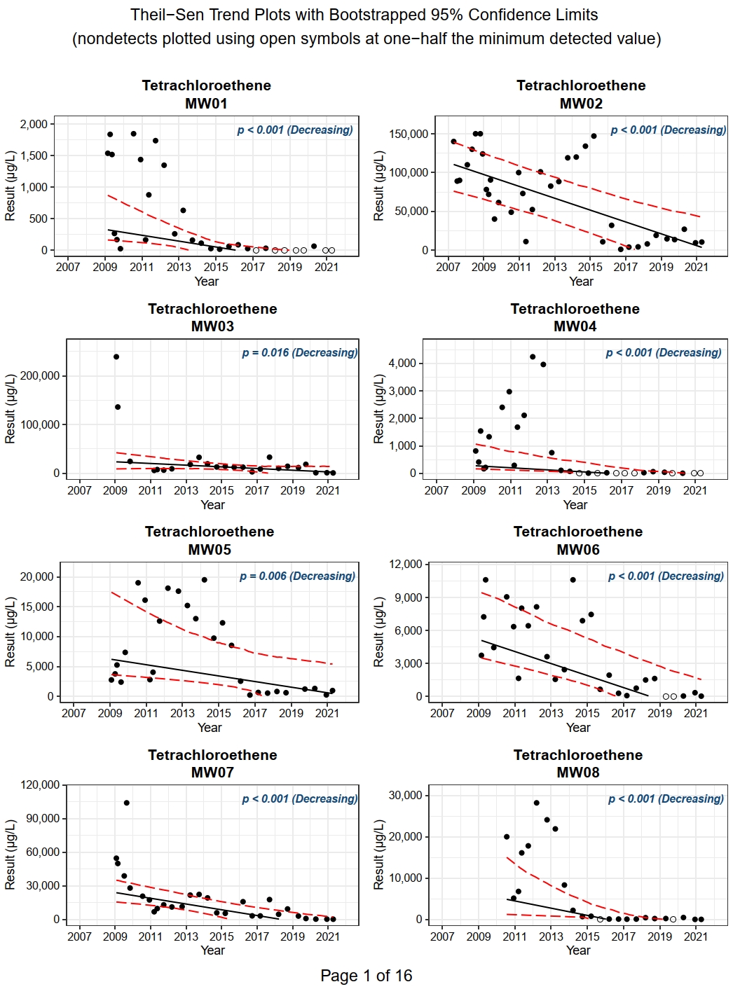
Trend Plots
The trend plots show the measured value of each parameter and location plotted against the sample collection date. Non-detects are shown as an open symbol plotted at one-half the minimum detected value in the dataset (when method = “KM”) or one-half the censoring limit (when method = “halflimit”). The trend plots include the Thiel-Sen trend line with nonparametric confidence bands constructed around the trend line using bootstrapping (USEPA 2009). In this method, the Theil-Sen trend is first computed using the sample data. Then a large number of bootstrap resamples are drawn from the original sample, and an alternate Theil-Sen trend is conducted on each bootstrap sample. Variability in these alternate trend estimates is then used to construct lower and upper confidence limits around the original trend.
The Theil-Sen trend line is only plotted for those location/parameter combinations where the Mann-Kendall test exhibits a statistically significant trend. The p-value and trend determination from the Mann-Kendall test is included with each trend plot.
Let’s create trend plots for all four VOCs in each individual monitoring well using the trendplots() function. The code shown below generated a pdf containing 124 trend plots; only the first of 16 pages of plots are shown.
# Generate trend plots
plots <- with(dat,
  trendplots(
    x = RESULT,
    detect = DETECTED,
    date = LOGDATE,
    loc = LOCID,
    param = PARAM,
    censor_limit = MDL,
    units_field = UNITS,
    alpha = 0.05,
    conf = 0.95
  )
)
As mentioned in the introduction to this section, individual plots can be saved as png files. The code for saving the individual trend plots is shown below.
# Save individual trend plots as pngs
# First, check that 'png' folder exists and if not, create it
output_dir <- file.path(getwd(), 'pngs')
if (!dir.exists(output_dir)) {
  dir.create(output_dir)
} else {
  print('Folder already exists!')
}

# Now save trend plots
for (i in 1:length(plots)) {
  file_name = paste0(getwd(), '/pngs/', 'trent_plot_', i, '.png')
  png(file_name, width = 6, height = 4, units = 'in', res = 300)
  plot(plots[[i]])
  dev.off()
}
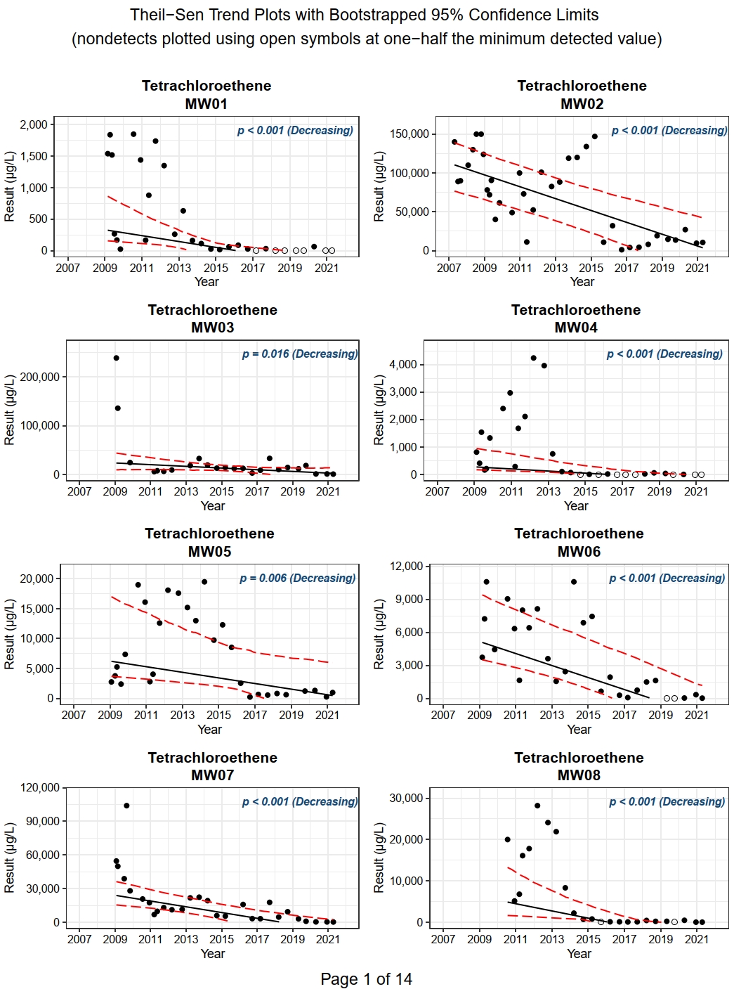
If there are a large number of wells and constituents, it may be useful to limit the trend plots to only those constituent/well pairs with a significantly significant trend in concentration as determined using the Mann-Kendall test. The code shown below generated a pdf containing 107 trend plots, corresponding to those constituent/well pairs with either an increasing or decreasing trend. Note that only the first of 14 pages of plots are shown.
# Get trend plots for location/parameter pairs where the Mann-Kendall test
# indicates either an increasing or decreasing trend
myvars <- c('LOCID', 'PARAM', 'TREND')
dat_trends <- merge(
  dat, trends[myvars],
  by = c('LOCID', 'PARAM'),
  all.x = TRUE
) %>%
filter(TREND %in% c('Increasing', 'Decreasing')) %>%
select(-c('TREND')) %>%
data.frame()

plots <- with(dat_trends,
  trendplots(
    x = RESULT,
    detect = DETECTED,
    date = LOGDATE,
    loc = LOCID,
    param = PARAM,
    censor_limit = MDL,
    units_field = UNITS,
    alpha = 0.05,
    conf = 0.95
  )
)
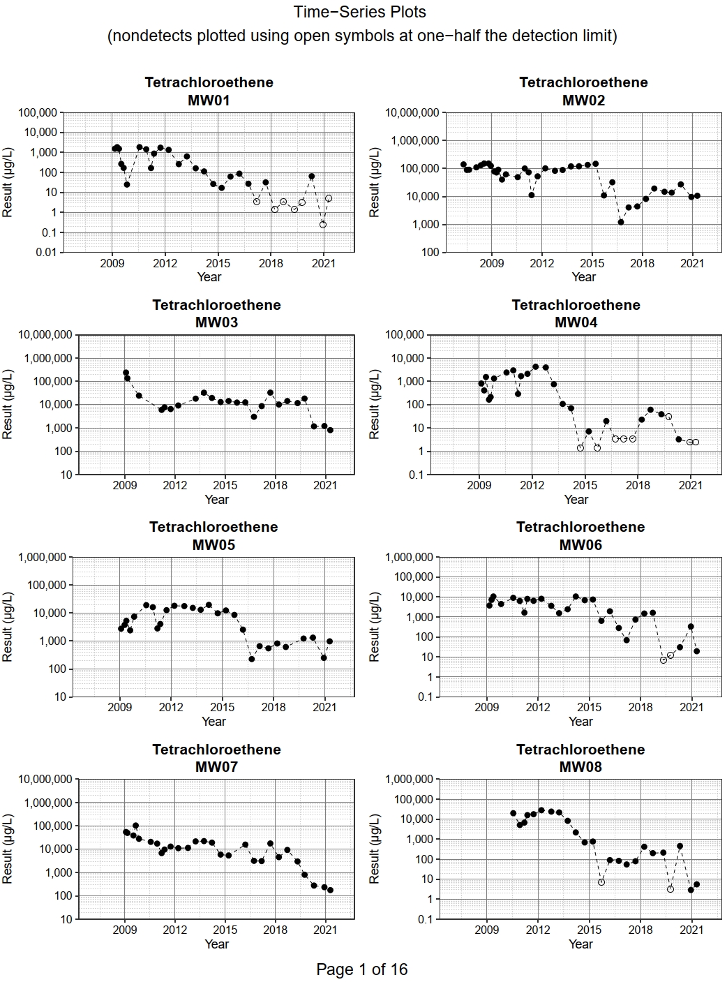
Time-Series Plots
The time-series plots show the measured value of each parameter and location plotted against the sample collection date. Non-detects are shown as an open symbol plotted at one-half the censoring limit, which is assigned in the function call by the user to the censor_limit variable. The user can select to create the time-series plots using a logarithm base 10 scale for the y-axis.
Let’s create time-series plots for all four VOCs in each individual monitoring well using the tsplots() function and selecting a log-scale for the y-axis. The code shown below generated a pdf containing 124 time-series plots; only the first of 16 pages of plots are shown.
plots <- with(dat,
  tsplots(
    x = RESULT,
    detect = DETECTED,
    date = LOGDATE,
    loc = LOCID,
    param = PARAM,
    censor_limit = MDL,
    units_field = UNITS,
    Log = TRUE,
    output_pdf = TRUE,
    pdf_name = 'TimeSeries_Plots',
    mst = 'Time-Series Plots',
    st = '(nondetects plotted using open symbols at one-half the detection limit)'
  )
)
As mentioned in the introduction to this section, individual plots can be saved as png files. The code for saving the individual time-series plots is shown below.
# Save individual time-series plots as pngs
# First, check that 'png' folder exists and if not, create it
output_dir <- file.path(getwd(), 'pngs')
if (!dir.exists(output_dir)) {
  dir.create(output_dir)
} else {
  print('Folder already exists!')
}

# Now save plots
for (i in 1:length(plots)) {
  file_name = paste0(getwd(), '/pngs/', 'ts_plot_', i, '.png')
  png(file_name, width = 6, height = 4, units = 'in', res = 300)
  plot(plots[[i]])
  dev.off()
}
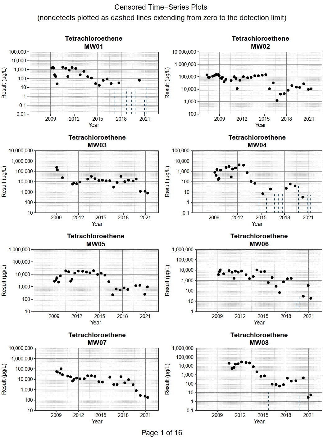
Censored Time-Series Plots
Time-series plots compare the values of a continuous variable (Y) plotted along the vertical axis as a function of time (X) on the horizontal axis. The paired X-Y values generally are visually inspected for patterns of correlation or trend. Unfortunately, when the Y variable is censored, such as when the data contain non-detects, the most common practice is to substitute one-half the censoring limit and plot the fabricated data as if it were measured. The result is a false impression that these values are actually known and that they are, in some cases, the same numerical value. For multiple censoring limits, plotting a fabricated value for non-detects may introduce an artifical pattern into the data. This may give a false impression when comparing observations.
Because censored values are known to be within an interval between zero and the censoring limit, representing these values by an interval, provides a visual depiction of what is actually known about the data. In censored time-series plots, censored or non-detect observations are shown as dashed vertical lines extending from zero to the censoring limit. Uncensored or detected observations are shown as single points. Censored time-series plots clearly illustrate the interval-censoring of the data. Censored observations are best shown as dashed vertical lines to emphasize that any one location within the interval is less likely than the single location shown for each detected observation (Helsel 2012).
Let’s create censored time-series plots for all four VOCs in each individual monitoring well using the cenplots() function and selecting a log-scale for the y-axis. The code shown below generated a pdf containing 124 censored time-series plots; only the first of 16 pages of plots are shown.
cen_plots <- with(dat,
  cenplots(
    x = RESULT,
    detect = DETECTED,
    date = LOGDATE,
    loc = LOCID,
    param = PARAM,
    censor_limit = MDL,
    units_field = UNITS,
    Log = TRUE,
    output_pdf = TRUE,
    pdf_name = 'Censored_TimeSeries_Plots',
    mst = 'Censored Time-Series Plots',
    st = '(nondetects plotted as dashed lines extending from zero to the detection limit)'
  )
)
Regression Analysis Plots
The regress() function fits a linear model of concentration-versus-time to each constituent/well pair data set. Regression can be performed either on the raw concentrations or the natural logarithm transformed concentration (referred to as log-linear regression). List-columns are used to store the results of the regression analysis, including the intercept, slope, coefficient of determination (r-squared), and the p-value that tests the null hypothesis that the slope is equal to zero. Regression plots can be produced showing the results of the regression analysis in relationship to the measured concentration data. If the limits variable is set to TRUE, lower and upper confidence limits defined by the level variable are shown for the fitted line on each plot. Regression is not performed if there are fewer than 6 detected results or if the data contain greater than 50% non-detects.
Let’s run log-linear regression for all four VOCs in each individual monitoring well using the regress() function. Because the non-detects must be assigned a value, we will use the RESULT2 from our original data frame. Recall that we assigned one-half the MDL to the non-detects in RESULT2. To provide an estimate of uncertainty, let’s use a two-sided 95% confidence interval. The code shown below generated a pdf containing 124 log-linear regression plots; only the first of 21 pages of plots are shown.
# Run log-linear regression
dfreg <- with(dat,
  regress(
    x = RESULT,
    detect = DETECTED,
    date = LOGDATE,
    loc = LOCID,
    param = PARAM,
    censor_limit = MDL,
    units_field = UNITS,
    Log = TRUE,
    Plot = TRUE,
    limits = TRUE,
    level = 0.95
  )
)

# Not run
# Save results to csv file
#outfile <- 'log-linear_regession.csv'
#write.table(dfreg, file = outfile, sep = ",",
#  row.names = F, col.names = T, append = F)
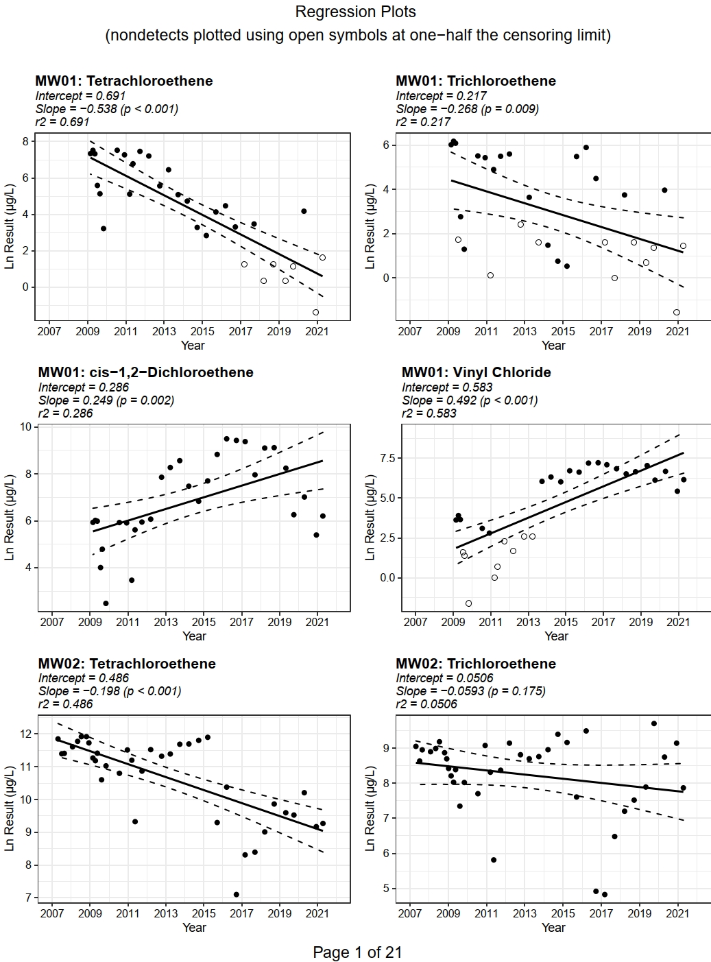
Combo Plots
Combo plots show the last measured value plotted as a function of the first-order attenuation rate for all monitoring locations for each parameter on a single plot. Plotting symbols are color-coded by the results of the Mann-Kendall test for monotonic trend. These plots are designed to provide a relatively complete data analysis summary of a single constituent across the entire monitoring well network in a single plot. The number of increasing and decreasing trends and the median attenutaion rate is provided at the top of each plot.
Let’s create combo plots for all four VOCs in each individual monitoring well using the comboplots() function and selecting a log-scale for the y-axis. The comboplots() function requires that the Mann-Kendall test and log-linear regression have been completed for the data set. The data frame containing the Mann-Kendall results is passed into the function using the tdf variable. The data frame containing the log-linear regression results is passed into the function using the rdf variable. This is shown in the code below.
# Generate combo plots using trends and dfreg
plots <- comboplots(
  tdf = trends,
  rdf = dfreg,
  labels = TRUE,
  logscale = TRUE
)
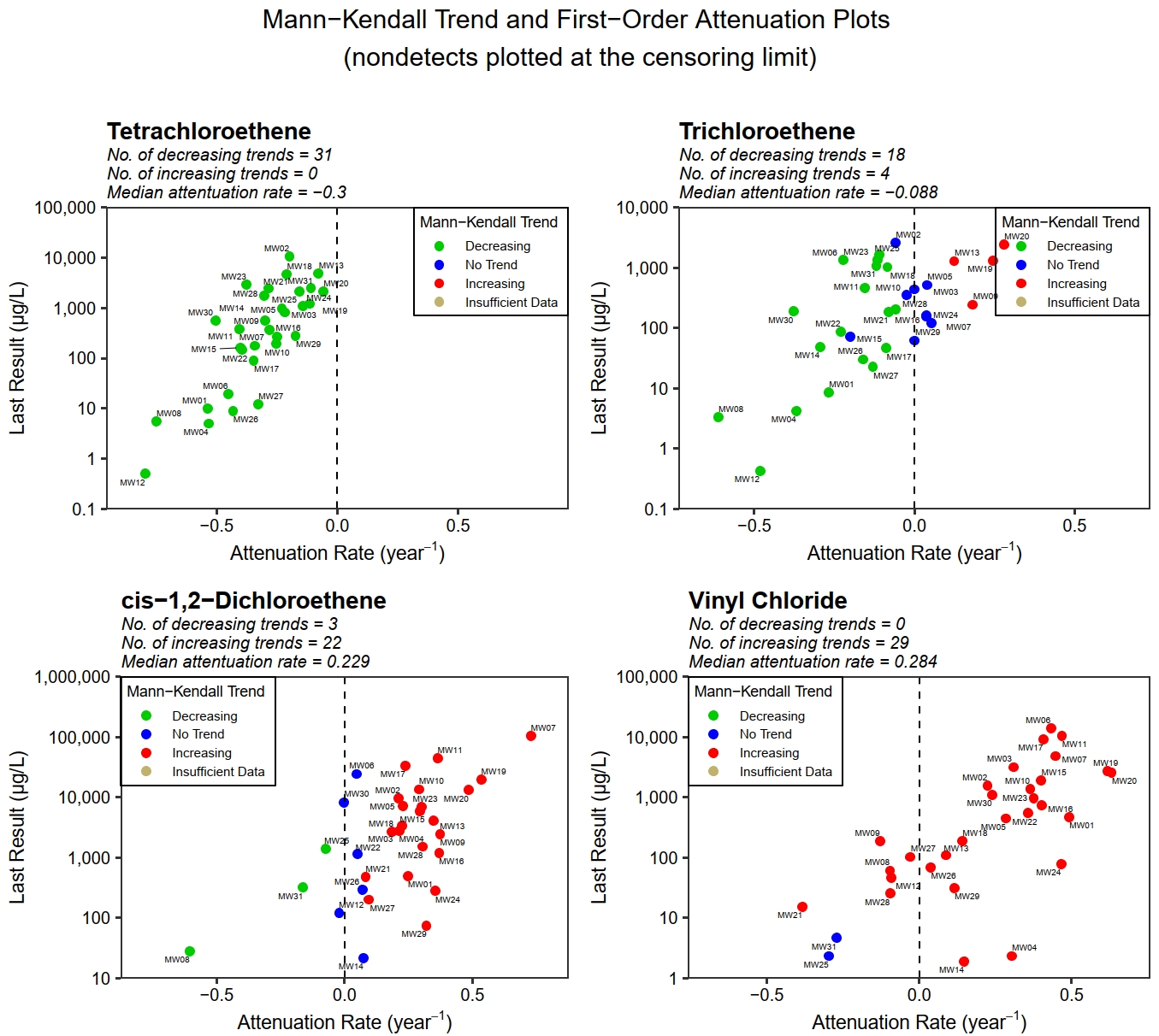
Based on the combo plots, it appears at this site that cis-1,2-dichloroethene and vinyl chloride are being produced via sequential degradation of tetrachloroethene and trichloroethene.
Conclusion
This rather verbose tutorial has been an introduction to the trendMK package and to the R statistical computing environment, at least to those not familiar with it. trendMK is intended to provide tools and insights to those scientists and engineers who have to analyze environmental groundwater monitoring data. trendMK incorporates statistical methods that have appeared in the environmental literature but are not commonly found in any statistical software package, or that are available but difficult to apply to a large data set, consisting of many wells and constituents. Although this tutorial does not discuss all the methods included in the trendMK package, it does provide the user an introduction upon which to further explore additional functionality of the package as well as R itself.
References
Akritas, M.G., S.S., Murphy, and M.P. LaValley. 1995. The Theil-Sen Estimator With Doubly Censored Data and Applications to Astronomy. J Am Stat Assoc. 90, 170-177.
Gilbert, R.O. 1987. Statistical Methods for Environmental Pollution Monitoring. Wiley, New York.
Helsel, D.R. 2012. Statistics for Censored Environmental Data Using Minitab and R, Second Edition. John Wiley and Sons, NJ.
Hollander, M. and D.A. Wolf. 1973. Nonparametric Statistical Methods. Wiley, New York.
Interstate Technology & Regulatory Council (ITRC). 2013. Groundwater Statistics and Monitoring Compliance: Statistical Tools for the Project Life Cycle. GSMC-1. December.
Kaplan, E.L. and O. Meier. 1958. Nonparametric Estimation from Incomplete Observations. J Am Stat Assoc. 53, 457-481.
Kendall, M.G. 1975. Rank Correlation Techniques, 4th ed. Charles Griffen. London.
Mann, H.B. 1945. Nonparametric Tests Against Trend. Econometrica, 13, 245-259.
Newell, C.J., I. Cowie, T.M. McGuire, and W.W. McNab, Jr. 2006. Multiyear Temporal Changes in Chlorinated Solvent Concentrations at 23 Monitored Natural Attenuation Sites. Journal of Environmental Engineering. 132, 653-663.
R Core Team. 2021. R: A language and environment for statistical computing. R Foundation for Statistical Computing, Vienna, Austria. http://www.R-project.org/.
Sen, P.K. 1968. Estimates of the Regression Coefficient Based on Kendall’s Tau. J Am Stat Assoc. 63, 1379-1389.
Theil, H. 1950. A Rank-Invariant Method of Linear and Polynomial Regression Analysis, I-III.Proc. Kon. Ned. Akad. v. Wetensch. A.53, 386-392, 521-525, 1397-1412.
Turnbull B.W. 1974. Nonparametric Estimation of a Survivorship Function With Doubly Censored Data. J Am Stat Assoc. 69, 169-173.
U.S. Environmental Protection Agency (USEPA). 2002. Calculation and Use of First-Order Rate Constants for Monitored Natural Attenuation Studies. EPA/540/S-02/500. U.S. Environmental Protection Agency, Washington, D.C.
USEPA. 2009. Statistical Analysis of Groundwater Monitoring Data at RCRA Facilities: Unified Guidance. EPA-530-R-09-007. Office of Resource Conservation and Recovery. Washington DC March.
USEPA. 2015. ProUCL Version 5.1 Technical Guide: Statistical Software for Environmental Applications for Data Sets with and without Nondetect Observations. EPA/600/R-07/041. U.S. Environmental Protection Agency, Office of Research and Development. Washington, DC. October.
- Posted on:
- March 13, 2022
- Length:
- 62 minute read, 13100 words
- See Also: