Testing Group Differences with Data Containing Non-detects
By Charles Holbert, Jacobs
September 13, 2019
Introduction
Often data from more than two groups needs to be evaluated, usually on the basis of a representative value from each group. In some of these cases, a “treatment” group is compared to a “control.” The control group may represent background, or historical conditions. The treatment group represents conditions where, for example, contaminant concentrations are suspected to be higher, or numbers of healthy organisms lower. When the evaluation is only concerned with differences in one direction, the test is referred to as a one-sided test. The key to a one-sided test is not in which direction the change is expected, but that there is only one direction expected. A two-sided test is concerned with differences in either direction, such as when comparing the concentrations in different locations with no control group.
For uncensored data, comparisons among groups are made using the parametric analysis of variance (ANOVA) and the nonparametric Kruskal-Wallis (KW) test. These tests determine whether the groups essentially belong to the same underlying population, or whether there are significant differences between the group means (in the case of parametric ANOVA) or the empirical distribution functions (in the case of the KW test). The nonparametric KW test does not assume the data follow any distribution, and therefore no transformations are required prior to computing the test.
When the KW test is applied to censored data, all observations below the highest reporting limit are assigned to the same value. When ranked, these observations become tied at the lowest rank. Data above the highest reporting limit are ranked using the same method as for uncensored data. However, when survival analysis techniques (Helsel 2012; Moore 2016) are used, there is no need to recensor the data using the highest reporting limit (RL). Because of this, survival analysis techniques provide greater power for data with multiple censoring limits.
Survival analysis encompasses a wide variety of methods for analyzing the timing of events. The prototypical event is death, which accounts for the name given to these methods. However, survival analysis is also appropriate for many other kinds of events, such as event-history analysis, divorce, child-bearing, unemployment, and reliability analysis. Most literature consider right censored survival data, but the same ideas can be used with left censored environmental data.
Data
In this example, we will use survival analysis techniques to test whether surface water concentrations differ in dissolved lead between various watersheds. In our data, Fourmile Creek represents our “control” (i.e., background). Concentrations of dissolved lead are all non-detect for one of the watersheds (Lost Creek) so let’s remove that data prior to conducting the group comparison.
First, we will load the comma-delimited data file and subset it so that we are only testing dissolved lead concentrations for all watersheds except Lost Creek. Then, we assign the RL to the non-detects and create a new variable indicating whether a result is censored, or non-detect (TRUE) or represents a detected value (FALSE).
# Load libraries
library(dplyr)
library(NADA)
library(multcomp)
library(survminer)

# Read data
datin <- read.csv('data/SurfaceWater_Bkgd_vs_Site.csv', header = T)

# Prep data
dat <- datin %>%
  mutate(
    LOGDATE = as.POSIXct(LOGDATE, format = '%m/%d/%Y'),
    RESULT2 = ifelse(DETECTED == 'Y', RESULT, RL),
    CENSORED = ifelse(DETECTED == 'N', TRUE, FALSE),
    WATERSHED = factor(WATERSHED)
  ) %>%
  filter(
    WATERSHED != 'Lost Creek' &
    PARAM == 'Lead, dissolved'
  ) %>%
    droplevels()
Let’s inspect the data using the cenfit() function in the NADA library. The cenfit() function computes descriptive statistics using the Kaplan-Meier (KM) product-limit estimator (Kaplan and Meier 1958) for data in each factor group. The KM method is a nonparametric method designed to incorporate data with multiple censoring levels and does not require an assumed distribution. Originally, this method was developed for analysis of right censored survival data where the KM estimator is an estimate of the survival curve, a complement of the cumulative distribution function. The KM method estimates a cumulative distribution function that indicates the probability for an observation to be at or below a reported concentration. The estimated cumulative distribution function is a step function that jumps up at each uncensored value and is flat between uncensored values.
# Review a summary of the data by group
with(dat, cenfit(obs = RESULT2, censored = CENSORED, groups = WATERSHED))
##                                n n.cen median         mean          sd
## WATERSHED=Beaver Creek        51    34 0.0005 0.0012297101 0.002713829
## WATERSHED=Elm Creek           34    25 0.0014 0.0032014760 0.006082457
## WATERSHED=Fourmile Creek      51    40 0.0002 0.0007995622 0.001779358
## WATERSHED=Lower Spring River  76    68 0.0004 0.0021118615 0.009324703
## WATERSHED=Neosho River        81    74     NA 0.0025210361 0.003708916
## WATERSHED=Tar Creek          419   202 0.0012 0.0178129895 0.029321270
Note that “NA” for the median lead concentration in the Neosho River means that the value is “below the RL”. We see that with the exception of the Tar Creek watershed, the data contain greater than 50 percent censored (non-detect) values.
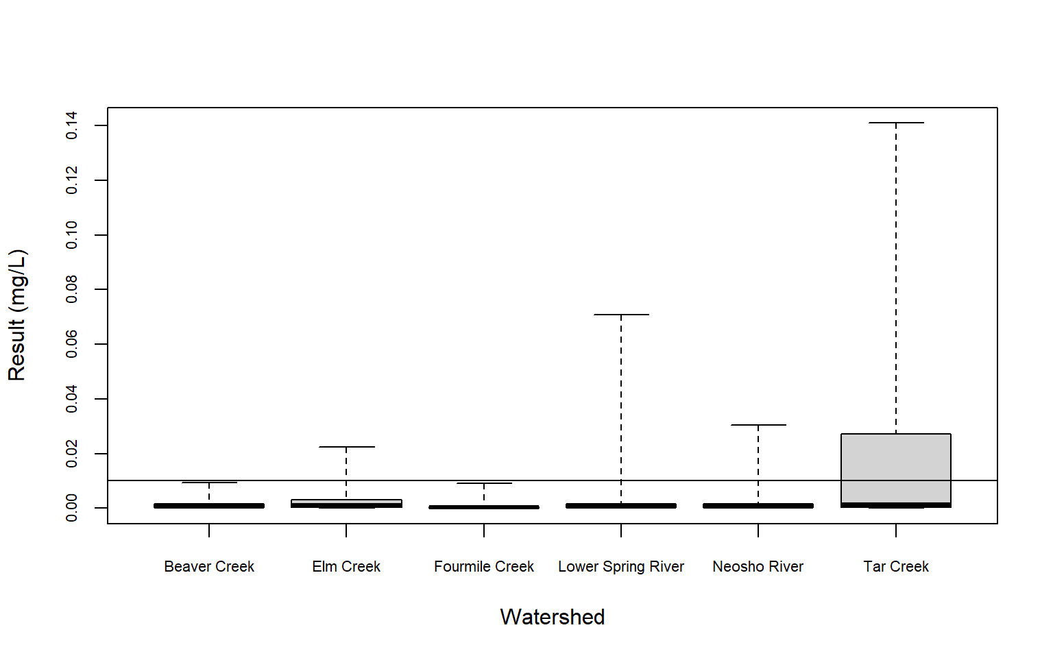
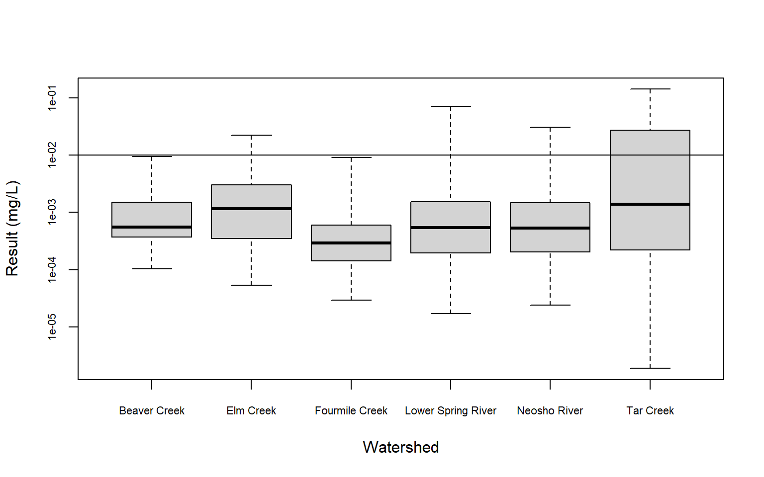
Now, let’s create censored box plots using both the raw concentrations and the log-transformed concentrations. Box plots are one of the most intuitive ways to visualize a dataset. They employ three percentiles (25th, 50th, and 75th) that define the central box. The relative positions of the percentiles show the center, spread, and skewness of the data. Censored observations can be incorporated into box plots by using the information in the proportion of data below the highest reporting limit. The highest censoring threshold is shown as a horizontal line on the plot and for this example, whiskers extend to the minimum and maximin data values. The 25th, 50th, and 75th percentiles have been estimated using robust Regression on Order Statistics (ROS), a method designed for analyzing multiply censored data (Helsel 2012).
# Create censored boxplot
with(dat,
  cenboxplot(
    obs = RESULT2, cen = CENSORED, group = WATERSHED,
    ylab = 'Result (mg/L)', xlab = 'Watershed',
    cex.axis = 0.7, log = FALSE
  )
)
# Create censored boxplot using logs
with(dat,
  cenboxplot(
    obs = RESULT2, cen = CENSORED, group = WATERSHED,
    ylab = 'Result (mg/L)', xlab = 'Watershed',
    cex.axis = 0.7, log = TRUE
  )
)
Testing Group Differences
Extensions of a linear rank test can be used for data with multiple censoring values (Prentice 1978). Different linear rank tests use different score functions, and some tests may be better than others at detecting a small shift in location, depending upon the true underlying distribution. The tests differ in the way different responses are weighted. The logrank test uses equal weighting across all responses while the other tests shift the heaviest weighting to the larger or smaller responses. Because of the different weighting patterns, they will often give quite different results. The following table describes the weighting scheme for the most common of these tests (NCSS 2019):
| Test | Weighting |
|---|---|
| Logrank | Equal weights across all responses |
| Gehan | Heavy weight on large responses |
| Tarone-Ware | Heavy weight on small responses |
| Peto-Peto | Little more weight on large responses |
| Modified Peto-Peto | Little more weight on large responses |
Millard and Deverel (1988) studied the behavior of several linear rank tests for censored data. The normal scores test using the Prentice and Marek computation of the normal scores was the best at maintaining the nominal type-I error rate in both equal and unequal sample sizes. When the sample sizes are equal, the Peto-Peto test (called Peto-Prentice in Millard and Deverel (1988)) with the asymptotic variance computation also maintained the nominal type I error rate and had a slightly higher power than the normal scores test. For data which look something like a lognormal distribution, the Tarone-Ware and Peto-Peto tests are reported to have more power than the logrank test (Helsel 2012).
Let’s compare our dissolved lead data using the survfitt function from the survival library. This function tests if there is a difference between two or more survival curves based on the KM estimate of survival using the G-rho family of tests (Harrington and Fleming 1982). With rho = 0 this is the logrank test, and with rho = 1 it is equivalent to the Peto-Peto modification of the Gehan-Wilcoxon test.
First, we need to create survival data using the Cen and flip functions in the NADA library. When used in concert with Cen, the flip function rescales left-censored data into right-censored data for use in the survival package routines.
# Create survival data using Cen and flip from NADA library
PbFlip <- with(dat, flip(Cen(RESULT2, CENSORED, type = "left")))

# Test if there is a difference between survival curves
survdiff(PbFlip ~ WATERSHED, data = dat, rho = 1)
## Call:
## survdiff(formula = PbFlip ~ WATERSHED, data = dat, rho = 1)
##
##                                N Observed Expected (O-E)^2/E (O-E)^2/V
## WATERSHED=Beaver Creek        51     9.70    16.37     2.715     3.729
## WATERSHED=Elm Creek           34     6.73     8.27     0.287     0.351
## WATERSHED=Fourmile Creek      51     6.32    20.31     9.641    14.090
## WATERSHED=Lower Spring River  76     5.44    17.80     8.581    11.199
## WATERSHED=Neosho River        81     5.41    18.66     9.402    12.250
## WATERSHED=Tar Creek          419   164.17   116.37    19.640    60.824
##
##  Chisq= 63.9  on 5 degrees of freedom, p= 2e-12
The p-value is <0.001, indicating there are differences in the dissolved lead concentration between at least two of the six watersheds. To determine which watersheds have different distributions of dissolved lead concentrations, let’s perform pairwise comparisons between group levels using the pairwise_survdiff function in the survminer library. When performing a large number of statistical tests, some p-values less than the typical significance level of 0.05 will occur purely by chance, even if all the null hypotheses are really true. The Bonferroni correction is one simple way to take this into account. However, adjusting the false discovery rate using the Benjamini-Hochberg (BH) procedure (Benjamini and Hochberg (1995) is a more powerful method to account for multiple comparisons. Thus, let’s us the BH method so that we have strong control of the family-wise error rate in our pairwise comparisons.
dat$PbFlip <- PbFlip
pairwise_survdiff(
  PbFlip ~ WATERSHED, data = dat,
  p.adjust.method = 'BH',
  rho = 1
)
##
## 	Pairwise comparisons using Peto & Peto test
##
## data:  dat and WATERSHED
##
##                    Beaver Creek Elm Creek Fourmile Creek Lower Spring River
## Elm Creek          0.1063       -         -              -
## Fourmile Creek     0.0505       0.0406    -              -
## Lower Spring River 0.8952       0.1391    0.2630         -
## Neosho River       0.4229       0.1269    0.4003         0.9273
## Tar Creek          0.0058       0.1200    4.4e-05        4.4e-05
##                    Neosho River
## Elm Creek          -
## Fourmile Creek     -
## Lower Spring River -
## Neosho River       -
## Tar Creek          4.4e-05
##
## P value adjustment method: BH
Based on a typical significance level of 0.05, we see that surface water concentrations of dissolved lead are different, on average, in the Elm Creek and Tar Creek watersheds than background (the Fourmile Creek watershed). The p-value for Elm Creek is only slightly below 0.05 at a value of 0.041, indicating dissolved lead concentrations in the Elm Creek watershed may likely be similar to background. For Tar Creek, the low p-value of <0.001 indicates that dissolved lead in this watershed is statistically different than background. These results are evident in the censored box plots, which show that dissolved lead concenatraions generally are higher in the Tar Creek watershed than the Fourmile Creek watershed.
Finally, let’s inspect the survival function plots for each watershed. A survival function plot is an empirical distribution function (edf) specifically developed for censored data. Survival function plots can be considered an edf plot flipped side to side, plotting (1 - p), the probabilities of exceedance of an observation (Helsel 2012). The edf is produced using the KM product-limit estimator (estimated survival distribution) of the flipped data. For left-censored data flipped and plotted using software for right-censored survival analysis, the largest observations are represented on the left side of the plot. Survival plots will typically label the x-axis as “Time” or “Survival Time.” Some survival analysis software will also compute the “cumulative failure time” probability p as well as the survival time (1 - p). “Failures” or “deaths” in survival analysis are the “detects” for environmental data.
By representing the dissolved lead data as interval censored, we can create cumulative failure time plots where the dissolved lead concentrations are plotted in the usual “low values on the left” format. This format is more familiar to environmental scientists than the reversed survival plot format.
dat$Pb_Left <- ifelse(dat$CENSORED == TRUE, -Inf, dat$RESULT2)
survdat <- with(dat, Surv(Pb_Left, RESULT2, type = 'interval2'))
fit <- survfit(survdat ~ WATERSHED, data = dat)
ggsurv <- ggsurvplot(fit, data = dat, fun = 'event')
ggpubr::ggpar(ggsurv, font.legend = list(size = 8, color = "black"))
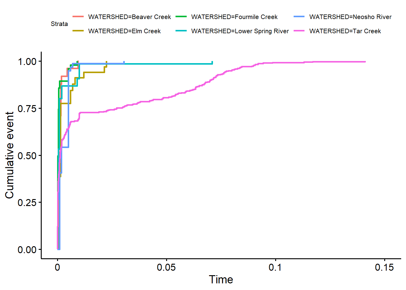
The cumulative failure time plots indicate that dissolved lead concentrations in the Tar Creek watershed, on average, are greater than concentrations in the Fourmile Creek watershed. Concentrations of dissolved lead in the other five watersheds appear similar to those in the Fourmile Creek watershed.
References
Benjamini, Y. and Hochberg, Y. 1995. Controlling the false discovery rate: a practical and powerful approach to multiple testing. Journal of the Royal Statistical Society Series B, 57, 289-300.
Harrington, D. P. and Fleming, T. R. 1982. A class of rank test procedures for censored survival data. Biometrika, 69, 553-566.
Helsel, D.R. 2012. Statistics for Censored Environmental Data Using Minitab and R. Second Edition. John Wiley and Sons, NJ.
Kaplan, E.L. and O. Meier. 1958. Nonparametric Estimation from Incomplete Observations. Journal of the American Statistical Association, 53, 457-481.
Millard, S.P. and Deverel, S.J. 1988. Nonparametric statistical methods for comparing two sites based on data with multiple non-detect limits. Water Resources Research, 24, 2087-2098..
Moore, D.F. 2016. Applied Survival Analysis Using R. Springer, Switzerland.
NCSS Statistical Software. 2019. Chapter 240: Nondetects-Data Group Comparisons. https://www.ncss.com/software/ncss/ncss-documentation/
Prentice, R.L. 1978. Linear rank tests with right censored data. Biometrika, 65, 167-179.
- Posted on:
- September 13, 2019
- Length:
- 11 minute read, 2247 words
- See Also: