Area Resource Survey Using Generalized Random Tessellation Stratified Sampling
By Charles Holbert, Jacobs
August 6, 2020
Introduction
Monitoring of biological and environmental processes are critical for understanding the health of our natural resources and making science-based management decisions. As with any ecological study, monitoring must be scaled to the variable and question being addressed. Monitoring should be done over a long enough time to incorporate the range of environmental conditions allowing for valid estimates of process variation. In addition to the time scale, it is equally important to consider spatial scales as part of the monitoring design. The collection and assessment of data may occur at various geographic scales, each requiring different sampling strategies and monitoring designs. Selection of monitoring locations is a critical part of the monitoring design; seldom is it possible to sample at all locations in a study area. In general, a goal in selecting monitoring locations is to obtain a “representative” sample. If the sample is not representative, then the information produced will not address the monitoring objectives - the data collected in the field are only as good as the locations selected for monitoring.
This factsheet illustrates a spatially balanced sampling design for an area resource using Generalized Random Tessellation Stratified (GRTS) sampling. An unstratified, equal probability design and a stratified, equal probability design will be developed using the spsurvey library (Kincaid 2020) within the R language and environment for statistical computing (R Core Team 2014).
Background
A variety of statistical books (e.g., Sarndal 1978; Cochran 1987; Thompson 1992; Lohr 1999) cover many aspects of sampling design, including clear definitions of the population of interest, sample units, the sample frame, and sample collection. Overton (1993) emphasizes probability sampling in the context of ecological monitoring, whereas Gilbert (1987) provides a theoretical account and illustration of sample design in an environmental context. Stevens and Olsen (2004) describe some of the attributes of environmental resources that affect environmental sampling design. Stevens and Urquhart (2000) discuss technical issues that arise with sample response designs in environmental settings.
Environmental processes are highly complex systems and as such, can be extremely challenging to monitor. They may change or move over time and/or space, with streams being less dynamic than air but more dynamic than soil. Furthermore, a reliable sampling frame for the target population is not always easy to produce, and it is typically only possible to sample a small proportion of a population. For large-scale environmental populations, the likelihood of spatially heterogeneity should be controlled through the sample design to ensure that the sample adequately represents the population.
Commonly used techniques for environmental sample design include convenience, judgmental, model-based, and probabilistic. The first two have been widely used in environmental management in general but have substantial deficiencies. A convenience sample is just that: there is no particular reason for selecting a location other than because it was easy to do so. The relationship between sample data and population characteristics is unknown, and there is no reasonable basis for extrapolating data from the sample to population characteristics. A judgmental sample is most often based on professional judgment founded on an informal synthesis of the investigator’s experience. One problematic issue is that if the locations truly are representative of central tendency, then the extremes are suppressed, and vice versa. Sample designs not based on probability lead to a number of problems including biased estimates of central tendency and variability. Model-based sample selection uses prior knowledge and theoretical population characteristics to choose sample locations. Model-based procedures can be very time consuming and expensive. The inference is based on the assumed completeness of knowledge and applicability of the model, and without demonstrated reliability based on extensive field data, model results may be limited in practical use.
The final method for selecting sample locations is a probability-based design, usually stratified random sampling. Prior knowledge and theoretical understanding can be incorporated into the process to focus the design. A statistical sampling design based on probabilistic sampling is the only way to ensure the selection of a representative sample from which can be drawn unbiased conclusions about the population as a whole. Probability-based sampling designs refers to the fact that every location in the population has a known, non-zero probability of being selected. These selection probabilities are determined by the sampling design and are, in turn, used to infer population characteristics from the selected sample.
Generalized Random Tessellation Stratified Sampling
As with most large-scale sample design problems, the central challenge is how to allocate sampling resources across space (and time) to maximize the information available, which can then be used to make reliable and credible inferences or predictions about the response(s) of interest. Spatial pattern is a dominant feature of environmental response variables. The pattern is shaped by geographic, meteorological, and anthropogenic stressors that all have pattern themselves. For large-scale environmental sampling, where the region of interest is too large to sample every location, spatially balanced sampling is a popular design. Spatially balanced designs ensure spatial coverage of the entire survey area, resulting in a sample that is representative of the population of interest.
There are many different methods of spatially balanced sampling designs (Wang et al. 2012). The most well known is Generalized Random Tessellation Stratified (GRTS) sampling (Stevens and Olsen 1999; Stevens and Olsen 2003; Stevens and Olsen 2004). In this design sample effort is spread evenly over the target region. The term “spread evenly” in this context means having coverage of survey effort over the region. The coverage from GRTS has a stochastic component rather than a fixed, regularly spaced internal as in a systematic sampling design. An invertible mapping technique is used to transform two-dimensional space into one-dimensional space. Then, a systematic sample is selected along the linear representation. Sampling location georeferences are generated from selecting points at regular intervals in this one-dimensional space (Brewer and Hanif 1983). The one-dimensional space is then mapped back to the two-dimensional original space. By maintaining the spatial properties of the original units, the resultant sample is balanced, with no one area being over-represented with high sample intensity nor under-represented with low sample intensity. Another advantage of GRTS samples is that they avoid the alignment problems and subsequent adverse effects on estimates that can occur with systematic sampling (Stevens and Olsen 2003).
The GRTS design was first designed for applications to large-scale monitoring and river systems. Since then it has been used in many applications. Some of the most recent examples are in forestry (Ackr et al. 2015), benthic surveys (Dunton et al. 2014), freshwater fish (Rodtka et al. 2015), and air quality associated with coal fires (Engle et al. 2013). The method can be used with point, linear, or areal features spanning one or more strata.
Area Resource
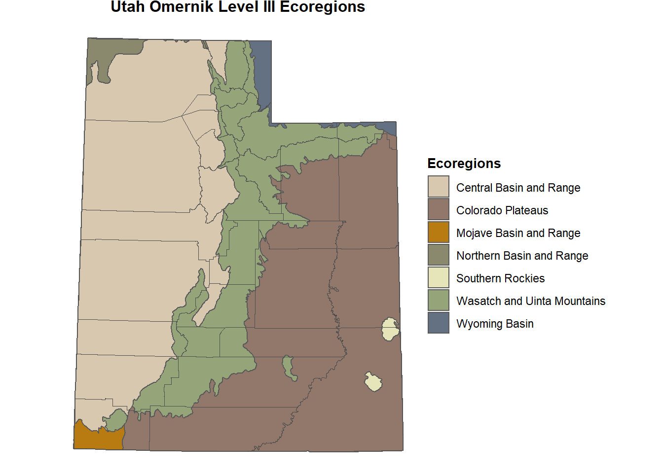
The area resource used in this example is based on the United States Environmental Protection Agency (USEPA) Omernik Level 3 Ecoregions (Omernik 1987) within Utah. The most common method of categorizing ecological variations across large landscapes is based on the ecoregion concept. Ecoregions are geographic delineations of landscapes containing ecosystems linked by similar climatic, geologic, soil, and landform characteristics. The primary characteristics used to delineate ecoregions vary depending on the overall goal of the individual or management agency. Therefore, ecoregions vary in their geographic extent and shape, but tend to generally identify similar geographies and ecosystems. Omernik Ecoregions were developed for the USEPA with the intent of generating regional water quality standards and thus are focused on hydrology.
Let’s load the area resource, which is included in the spsurvey library as a shapefile.
# Load libraries
library(spsurvey)
library(sf)
library(ggplot2)

# Read shapefile objects
load(file = 'data/UT_ecoregions.rda')
counties <- st_read("shapes/Counties_lines.shp", quiet = TRUE)

# Inspect data
head(UT_ecoregions)
## Simple feature collection with 6 features and 3 fields
## Geometry type: MULTIPOLYGON
## Dimension:     XY
## Bounding box:  xmin: -1574643 ymin: 1629173 xmax: -1085382 ymax: 2250764
## Projected CRS: NAD83 / Conus Albers
##   Level3                  Level3_Nam     Area_ha                       geometry
## 1     80    Northern Basin and Range 1.42202e+11 MULTIPOLYGON (((-1317868 22...
## 2     18               Wyoming Basin 1.33312e+11 MULTIPOLYGON (((-1128931 20...
## 3     13     Central Basin and Range 3.09949e+11 MULTIPOLYGON (((-1487359 21...
## 4     19 Wasatch and Uinta Mountains 4.47240e+10 MULTIPOLYGON (((-1288590 22...
## 5     20           Colorado Plateaus 1.26379e+11 MULTIPOLYGON (((-1087925 20...
## 6     21            Southern Rockies 5.40909e+08 MULTIPOLYGON (((-1133832 18...
The shapefile is a multpolygon feature containing 4 attributes. The ecoregion is contained in the attribute named “Level3_Nam” and includes seven unique values. The ecoregion area is measured in hectares and is contained in the attribute named “Area_ha”. Let’s calculate the total area for each ecoregion and the total area for all ecoregions.
# Summarize area by ecoregion
area_summary <- with(UT_ecoregions, tapply(Area_ha, Level3_Nam, sum))
area_summary <- round(addmargins(area_summary), 0)
data.frame(area_summary)
##                             area_summary
## Central Basin and Range     309949000000
## Colorado Plateaus           126379000000
## Mojave Basin and Range      129599000000
## Northern Basin and Range    142202000000
## Southern Rockies               946443000
## Wasatch and Uinta Mountains  45693759000
## Wyoming Basin               133312000000
## Sum                         888081202000
The coordinate system of the shapefile is given in NAD83 using the Albers equal-area conic projection. Let’s reproject the shapefile to UTM Zone 12N, NAD83 and then create a map showing the ecoregions.
# Reproject UT_ecoregions shapefile to UTM Zone 12N, NAD83
UT_ecoregions_sp <- st_transform(UT_ecoregions, crs = 3742)

# Create vector of colors
cols <- c(
  "#D8C8AF",
  "#92786B",
  "#B77B11",
  "#8B896D",
  "#E6E5BA",
  "#95A579",
  "#647183"
)

# Plot UT ecoregions
ggplot() +
  geom_sf(data = UT_ecoregions_sp, aes(fill = Level3_Nam)) +
  geom_sf(data = counties, color = 'grey30', size = 0.2) +
  coord_sf() +
  labs(title = "Utah Omernik Level III Ecoregions") +
  scale_fill_manual(values = cols) +
  guides(fill = guide_legend(title = "Ecoregions")) +
  theme_void() +
  theme(plot.title = element_text(margin = margin(b = 2), size = 12,
                                  hjust = 0.5, color = "black",
                                  face = quote(bold)),
        legend.title = element_text(size = 10, color = "black",
                                    face = quote(bold)))
Unstratified Sample Design
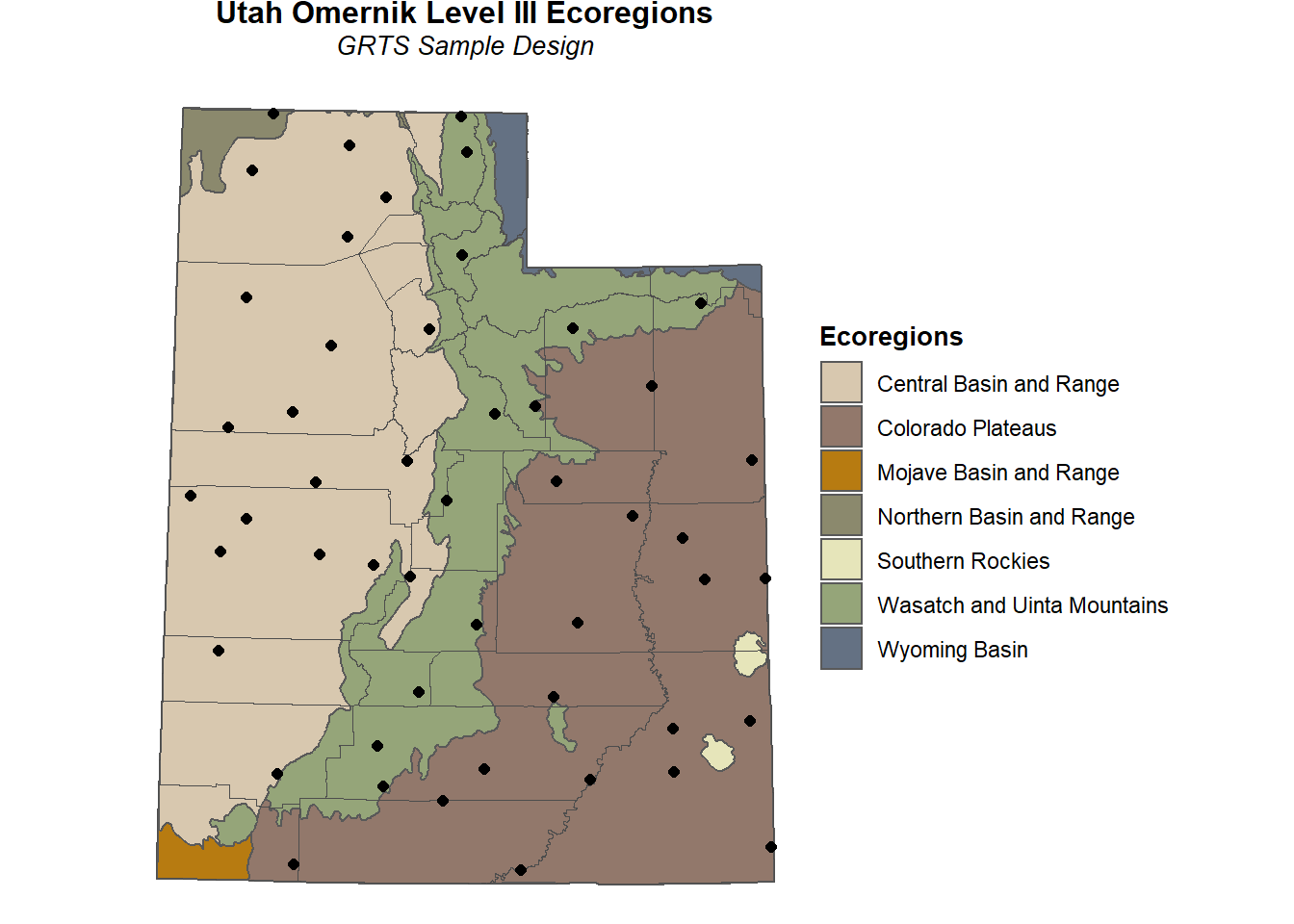
Let’s develop an unstratified, equal probability sample design for the Utah ecoregions. The initial step is to create a list that contains information for specifying the survey design. Because the survey design is unstratified, the list contains a single list item that includes two items: panel, which is used to specify the sample size for each panel, and seltype, which is used to input the type of random selection for the design. For this example, panel is assigned a single value named “PanelOne” that is set equal to 50, and seltype is assigned the value “Equal”, which indicates equal probability selection. The first six rows of the sample design is provided below.
# Create the design list
set.seed(4447864)
Equaldsgn <- list(None = list(panel = c(PanelOne = 50),
                              seltype = "Equal"))

# Select the sample
Equalsites <- grts(design     = Equaldsgn,
                   DesignID   = "EQUAL",
                   type.frame = "area",
                   src.frame  = "sf.object",
                   sf.object  = UT_ecoregions_sp,
                   maxlev     = 5,
                   shapefile  = FALSE)
##
## Stratum: None
## Current number of levels: 3
## Current number of levels: 4
## Final number of levels: 4
# Print the initial six lines of the survey design
head(Equalsites)
##           coordinates   siteID   xcoord  ycoord mdcaty        wgt stratum
## 1 (425938.2, 4494321) EQUAL-01 425938.2 4494321  Equal 4395061373    None
## 2 (388127.9, 4193986) EQUAL-02 388127.9 4193986  Equal 4395061373    None
## 3   (452507, 4621437) EQUAL-03 452507.0 4621437  Equal 4395061373    None
## 4 (541760.3, 4169993) EQUAL-04 541760.3 4169993  Equal 4395061373    None
## 5 (517511.4, 4384661) EQUAL-05 517511.4 4384661  Equal 4395061373    None
## 6 (275037.1, 4334200) EQUAL-06 275037.1 4334200  Equal 4395061373    None
##      panel EvalStatus EvalReason Level3                  Level3_Nam     Area_ha
## 1 PanelOne    NotEval                13     Central Basin and Range 3.09949e+11
## 2 PanelOne    NotEval                19 Wasatch and Uinta Mountains 4.47240e+10
## 3 PanelOne    NotEval                19 Wasatch and Uinta Mountains 4.47240e+10
## 4 PanelOne    NotEval                20           Colorado Plateaus 1.26379e+11
## 5 PanelOne    NotEval                20           Colorado Plateaus 1.26379e+11
## 6 PanelOne    NotEval                13     Central Basin and Range 3.09949e+11
A summary of the unstratified, equal probability sample design is given as:
# Print the survey design summary
summary(Equalsites)
##
##
## Design Summary: Number of Sites
##
## stratum
## None  Sum
##   50   50
Now that we have the unstratified, equal probability sample design, we can plot the sample locations on the area resource map. The unstratified, equal probability samples are shown as black circles.
# Plot sf with points
p <- ggplot() +
       geom_sf(data = UT_ecoregions_sp,
               aes(fill = Level3_Nam)) +
       geom_sf(data = counties, color = 'grey30', size = 0.2) +
       coord_sf() +
       labs(title = "Utah Omernik Level III Ecoregions",
            subtitle = "GRTS Sample Design") +
       theme_void() +
       scale_fill_manual(values = cols) +
       guides(fill = guide_legend(title = "Ecoregions")) +
       theme(plot.title = element_text(margin = margin(b = 2), size = 12,
                                       hjust = 0.5, color = "black",
                                       face = quote(bold)),
             plot.subtitle = element_text(margin = margin(b = 4), size = 10,
                                          hjust = 0.5, color = "black",
                                          face = quote(italic)),
             legend.title = element_text(size = 10, color = "black",
                                         face = quote(bold)))

# Add sampling points
pts <- data.frame(x = Equalsites$xcoord, y = Equalsites$ycoord)
p <- p + geom_point(data = pts, aes(x = x, y = y),
                    shape = 16, size = 1.8, color = "black")
p
Stratified Sample Design
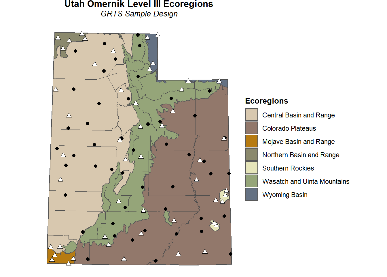
Let’s develop a stratified, equal probability sample design where the ecoregions are used to identify strata. We will create a Stratdsgn list to identify the seven ecoregions (i.e., strata), where the names match the unique values of the ecoregion attribute of the shapefile. Each list in Stratdsgn contains two items: panel and seltype. We will assign panel a value of either 5 or 10, and seltype is assigned “Equal”, which indicates equal probability selection. The first six rows of the sample design is provided below.
# Create the design list
Stratdsgn <- list(
  "Central Basin and Range"     = list(panel = c(PanelOne = 10), seltype = "Equal"),
  "Colorado Plateaus"           = list(panel = c(PanelOne = 10), seltype = "Equal"),
  "Mojave Basin and Range"      = list(panel = c(PanelOne =  5), seltype = "Equal"),
  "Northern Basin and Range"    = list(panel = c(PanelOne =  5), seltype = "Equal"),
  "Southern Rockies"            = list(panel = c(PanelOne =  5), seltype = "Equal"),
  "Wasatch and Uinta Mountains" = list(panel = c(PanelOne = 10), seltype = "Equal"),
  "Wyoming Basin"               = list(panel = c(PanelOne =  5), seltype = "Equal")
)

# Select the sample
Stratsites <- grts(design     = Stratdsgn,
                   DesignID   = "STRATIFIED",
                   type.frame = "area",
                   src.frame  = "sp.object",
                   sp.object  = UT_ecoregions_sp,
                   stratum    = "Level3_Nam",
                   maxlev     = 5,
                   shapefile  = TRUE)
##
## Stratum: Central Basin and Range
## Current number of levels: 2
## Current number of levels: 3
## Final number of levels: 3
##
## Stratum: Colorado Plateaus
## Current number of levels: 2
## Current number of levels: 3
## Final number of levels: 3
##
## Stratum: Mojave Basin and Range
## Current number of levels: 2
## Final number of levels: 2
##
## Stratum: Northern Basin and Range
## Current number of levels: 2
## Current number of levels: 3
## Final number of levels: 3
##
## Stratum: Southern Rockies
## Current number of levels: 2
## Current number of levels: 3
## Final number of levels: 3
##
## Stratum: Wasatch and Uinta Mountains
## Current number of levels: 2
## Current number of levels: 3
## Current number of levels: 4
## Final number of levels: 4
##
## Stratum: Wyoming Basin
## Current number of levels: 2
## Current number of levels: 3
## Final number of levels: 3
# Print the initial six lines of the survey design
head(Stratsites)
##           coordinates        siteID   xcoord  ycoord mdcaty        wgt
## 1 (407588.8, 4514247) STRATIFIED-01 407588.8 4514247  Equal 8206469083
## 2 (344545.2, 4576411) STRATIFIED-02 344545.2 4576411  Equal 8206469083
## 3 (268729.9, 4358271) STRATIFIED-03 268729.9 4358271  Equal 8206469083
## 4 (418518.8, 4347903) STRATIFIED-04 418518.8 4347903  Equal 8206469083
## 5 (388795.9, 4607967) STRATIFIED-05 388795.9 4607967  Equal 8206469083
## 6 (261926.1, 4299130) STRATIFIED-06 261926.1 4299130  Equal 8206469083
##                   stratum    panel EvalStatus EvalReason Level3     Area_ha
## 1 Central Basin and Range PanelOne    NotEval                13 3.09949e+11
## 2 Central Basin and Range PanelOne    NotEval                13 3.09949e+11
## 3 Central Basin and Range PanelOne    NotEval                13 3.09949e+11
## 4 Central Basin and Range PanelOne    NotEval                13 3.09949e+11
## 5 Central Basin and Range PanelOne    NotEval                13 3.09949e+11
## 6 Central Basin and Range PanelOne    NotEval                13 3.09949e+11
A summary of the stratified, equal probability sample design is given as:
# Print the survey design summary
summary(Stratsites)
##
##
## Design Summary: Number of Sites
##
## stratum
##     Central Basin and Range           Colorado Plateaus
##                          10                          10
##      Mojave Basin and Range    Northern Basin and Range
##                           5                           5
##            Southern Rockies Wasatch and Uinta Mountains
##                           5                          10
##               Wyoming Basin                         Sum
##                           5                          50
Now that we have the stratified, equal probability sample design, we can plot the sample locations on the area resource map. The stratified, equal probability samples are shown as white triangles while the unstratified, equal probability samples are shown as black circles.
# Plot points on map
pts <- data.frame(x = Stratsites$xcoord, y = Stratsites$ycoord)
p <- p + geom_point(data = pts, aes(x = x, y = y),
                    shape = 24, size = 2, fill = "white", color = "black")
p
Conclusion
Care must be exercised when using non-random sample selection methods because the samples may not be representative of the entire population as a whole, and inference cannot extend beyond the sample population. While a systematic sample design can achieve complete spatial balance, it lacks randomization that is desirable in statistical sample designs and it is difficult to apply when the units being selected for sampling are not contiguous within the study area (e.g., selecting lakes or wetlands to sample). The GRTS method can be used to provide a spatially balanced, probability sample with design-based, unbiased variance estimators with a minimum sample size. Simulations by Lackey and Stein (2013) showed significantly increased precision and reduced bias with GRTS sampling compared to simple random sampling. However, if the estimation of spatial autocorrelation of population parameters is desired (i.e., for geostatistical techniques), spatially balanced sampling may not be the best option.
References
Acker S.A., J.R. Boetsch, M. Bivin, L. Whiteaker, C. Cole, and T. Philippi. 2015. Recent tree mortality and recruitment in mature and old-growth forests in western Washington. Forest Ecology Management, 336:109-118.
Brewer, K. R. W. and M. Hanif. 1983. Sampling With Unequal Probabilities, New York, Springer-Verlag.
Cochran, W. G. 1987. Sampling Techniques, 3rd Edition. John Wiley & Sons, New York.
Dunton K.H., J.M. Grebmeier, and J.H. Trefry. 2014. The benthic ecosystem of the northeastern Chukchi Sea: An overview of its unique biogeochemical and biological characteristics. Deep Sea Research Part II, 102:1-8.
Engle M.A., R.A. Olea, J.M.K. O’Keefe, J.A. Hower, and N.J. Geboy. 2013. Direct estimation of diffuse gaseous emissions from coal fires: Current methods and future directions. Int J Coal Geol, 112:164-172.
Gilbert, R. O. 1987. Statistical Methods for Environmental Pollution Monitoring. Van Nostrand Reinhold, New York.
Kincaid, T. 2020. https://cran.r-project.org/web/packages/spsurvey/vignettes/Area_Design.html.
Lackey, L.G. and E.D. Stein. 2013. Evaluation of design-based sampling options for monitoring stream and wetland extent and distribution in California. Wetlands, 33:717-725.
Lohr, S. L. 1999. Sampling: Design and Analysis. Duxbury Press, Pacific Grove, California.
Olsen, A. R., J. Sedransk, E. Edwards, C. A. Gotway, and W. Liggett. 1999. Statistical issues for monitoring ecological and natural resources in the United States. Environmental Monitoring and Assessment, 54:1-45.
Omernik, J.M. 1987. Ecoregions of the conterminous United States. Annals of the Association of Amercian Geographers, 77:118-125.
Overton, W.S. 1993. Probability sampling and population inference in monitoring programs. In Environmental Monitoring with GIS, M.R. Goodchild, S.O. Parks, and C.T. Steyaert, Eds. Oxford University Press, NY, 470-480.
R Core Team. 2014. R: A language and environment for statistical computing. R Foundation for Statistical Computing, Vienna, Austria. http://www.R-project.org/.
Rodtka M.C., C.S. Judd, P.K.M. Aku, and K.M. Fitzsimmons. 2015. Estimating occupancy and detection probability of juvenile bull trout using backpack electrofishing gear in a west-central Alberta watershed. Can J Fish Aquat Sc, 72:742-750.
Sarndal, C. 1978. Design-based and model-based inference for survey sampling. Scandinavian Journal of Statistics, 5:27-52.
Stehman, S. V., and W. S. Overton. 1994. Environmental sampling and monitoring. Pages 263?306 in G. P. Patil and C. R. Rao, editors. Handbook of Statistics, Volume 12. Elsevier Science, Amsterdam, The Netherlands.
Stevens D.L. and A.R. Olsen. 1999. Spatially restricted surveys over time for aquatic resources. J Agr Biol Envir Stat. 4:415-428.
Stevens D.L. and A.R. Olsen. 2004. Spatially balanced sampling of natural resources. J Am Stat Assoc., 99:262-278.
Stevens D.L. and A.R. Olsen. 2003. Variance estimation for spatially balanced samples of environmental resources. Environ Metrics, 14:593-610.
Stevens, D.L., Jr., and N.S. Urquhart. 2000. Response designs and support regions in sampling continuous domains. Environmetrics, 11:13-41.
Thompson, S. K. 1992. Sampling. John Wiley & Sons, New York.
Wang J.F., A. Stein, B.B. Gao, and Y. Ge. 2012. A review of spatial sampling. Spatial Statistics, 2:1-14.
- Posted on:
- August 6, 2020
- Length:
- 17 minute read, 3417 words
- See Also: