Introduction

Landscapes contain complex spatial patterns in the distribution of resources that vary over time. Quantifying these patterns and their dynamics is the purview of landscape pattern analysis. Landscape pattern consists of two essential components: 1) landscape composition, or the types of land uses and land covers present and their relative proportions, and 2) landscape structure, or the spatial arrangement of these landscape elements. The basic unit in landscape pattern analysis is land cover-land use. Although changes in landscape pattern invariably impact the local landscape, the consequences can have global ramifications (Foley et al. 2005).

The main idea of pattern-based analysis is that any categorical raster dataset can be described using some spatial signitures. Spatial patterns in categorical raster data are most often described by landscape metrics. Landscape metrics consist of a set of algorithms for deriving neighborhood-based spatial characteristics of land cover patches, classes, or an entire landscape mosaic (McGarigal and Marks 1995). Despite the fact that methods and metrics for analysing land use change are well developed, calculating and visualizing them over large geographic areas, at high spatial and temporal resolutions, poses significant challenges. However, increased availability of spatial data and satellite imagery, combined with advances in computing power, are creating unprecedented opportunities for landscape pattern analysis.

The focus of this post is on the spatial analysis of landscapes using the R programming environment for statistical analysis and visualization (R Core Team 2020). Base R includes many functions that can be used for reading, visualising, and analysing spatial data. These base R functions are complemented by contributed packages for spatial pattern analysis and for quantifying landscape characteristics. For example, the landscapemetrics package (Hesselbarth et al. 2019) is an R package for calculating landscape metrics for categorical landscape patterns based on the main concepts from FRAGSTATS (McGarigal et al. 2012). It includes procedures for removing existing metric implementation errors, adding new landscape metrics, enabling landscape visualization, and allowing for calculations on large input data. A particular advantage is the ability to integrate this package with other R packages for spatial analysis, so it is possible to download spatial data, process it, calculate landscape metrics, and visualize them within one software programming tool.

Data

The quantitative analysis of the landscape spatial pattern for two U.S. cities will be carried out by using Landsat-8 remote sensing data. The majority of Landsat data are delivered at a pixel size of 30 meters (m). This pixel size prevents fine-scale mapping of surface features; however, it accurately captures landscape-scale characteristics while avoiding the significant computational requirements associated with hyper-spatial and hyper-spectral sensors (Young et al. 2017). Generally, the spatial features of interest are those relating to fragmentation, complexity, size, and shape of the patches. In this context, satellite images make it possible to gather consistent and complete spatial data for very large areas and may be considered a very useful tool for measuring landscape patterns, because they provide a digital mosaic of the spatial arrangement of land covers (Chuvieco 1999).

Landsat-8 is the most recently launched Landsat satellite and carries the Operational Land Imager (OLI) and the Thermal Infrared Sensor (TIRS) instruments (USGS 2021). The OLI includes nine spectral bands:

• B1 Ulra-blue
• B2 Blue
• B3 Green
• B4 Red
• B5 Near-Infrared (NIR)
• B6 Shortwave infrared (SWIR)
• B7 SWIR 2
• B8 Panchromatic (PAN)
• B9 Cirrus

TIRS collects data for two more narrow spectral bands in the thermal region.

Bozeman, Montana

This analysis will use the Landsat-8 scene of Bozeman, Montana on July 21, 2020 with a 30 m resolution for the RGB, NIR, and SWIR bands. Let’s import the RGB color bands as individual ‘RasterLayer’ objects. After importing the bands, we will combine the RasterLayer objects and visualize the satellite image.

\vspace{8pt}

# Load libraries
library(raster)
library(sf)

# blue
b2 <- raster('data/Landsat8_Bozeman/LC08_L1TP_039028_20200721_20200807_01_T1_B2.tif')

# green
b3 <- raster('data/Landsat8_Bozeman/LC08_L1TP_039028_20200721_20200807_01_T1_B3.tif')

# red
b4 <- raster('data/Landsat8_Bozeman/LC08_L1TP_039028_20200721_20200807_01_T1_B4.tif')

# Combine objects and visualize satellite image
landsatRGB <- stack(b4, b3, b2)  # order is important
plotRGB(landsatRGB, stretch = 'lin')

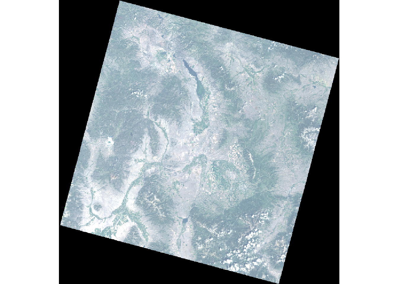
Figure 1: Landsat-8 true color composite (RGB) of Bozeman area (Source: U.S. Geological Survey).

Now, let’s import all 5 bands from the satellite data as a ‘RasterStack’ object.

# Get file names
filenames <- paste0(
  'data/Landsat8_Bozeman/LC08_L1TP_039028_20200721_20200807_01_T1_B',
  1:5,
  '.tif'
)

# Create stack
landsat <- stack(filenames)

# Rename bands
names(landsat) <- c('ultra-blue', 'blue', 'green', 'red', 'NIR')

Let’s check the coordinate reference system of the landsat stack.

# Check coordinate reference system of 'landsat'  
crs(landsat)

## Coordinate Reference System:
## Deprecated Proj.4 representation:
##  +proj=utm +zone=12 +datum=WGS84 +units=m +no_defs 
## WKT2 2019 representation:
## PROJCRS["WGS 84 / UTM zone 12N",
##     BASEGEOGCRS["WGS 84",
##         DATUM["World Geodetic System 1984",
##             ELLIPSOID["WGS 84",6378137,298.257223563,
##                 LENGTHUNIT["metre",1]]],
##         PRIMEM["Greenwich",0,
##             ANGLEUNIT["degree",0.0174532925199433]],
##         ID["EPSG",4326]],
##     CONVERSION["UTM zone 12N",
##         METHOD["Transverse Mercator",
##             ID["EPSG",9807]],
##         PARAMETER["Latitude of natural origin",0,
##             ANGLEUNIT["degree",0.0174532925199433],
##             ID["EPSG",8801]],
##         PARAMETER["Longitude of natural origin",-111,
##             ANGLEUNIT["degree",0.0174532925199433],
##             ID["EPSG",8802]],
##         PARAMETER["Scale factor at natural origin",0.9996,
##             SCALEUNIT["unity",1],
##             ID["EPSG",8805]],
##         PARAMETER["False easting",500000,
##             LENGTHUNIT["metre",1],
##             ID["EPSG",8806]],
##         PARAMETER["False northing",0,
##             LENGTHUNIT["metre",1],
##             ID["EPSG",8807]]],
##     CS[Cartesian,2],
##         AXIS["(E)",east,
##             ORDER[1],
##             LENGTHUNIT["metre",1]],
##         AXIS["(N)",north,
##             ORDER[2],
##             LENGTHUNIT["metre",1]],
##     USAGE[
##         SCOPE["Engineering survey, topographic mapping."],
##         AREA["Between 114°W and 108°W, northern hemisphere between equator and 84°N, onshore and offshore. Canada - Alberta; Northwest Territories (NWT); Nunavut; Saskatchewan. Mexico. United States (USA)."],
##         BBOX[0,-114,84,-108]],
##     ID["EPSG",32612]]

Let’s import a polygon of the city boundaries and transform the coordinate reference system to match that of the landsat object.

# Import polygon of city boundaries  
sgshp <- st_read("data/Shapefiles/Bozeman.shp")

## Reading layer `Bozeman' from data source 
##   `C:\Users\cholbert\mywebsite\content\blog\landscape_pattern_analysis\data\shapefiles\Bozeman.shp' 
##   using driver `ESRI Shapefile'
## Simple feature collection with 1 feature and 3 fields
## Geometry type: POLYGON
## Dimension:     XY
## Bounding box:  xmin: 473832.8 ymin: 155069.4 xmax: 484420.3 ymax: 166098.3
## Projected CRS: NAD83 / Montana

# Check coordinate reference system 
crs(sgshp)

## Coordinate Reference System:
## Deprecated Proj.4 representation:
##  +proj=lcc +lat_0=44.25 +lon_0=-109.5 +lat_1=49 +lat_2=45 +x_0=600000
## +y_0=0 +datum=NAD83 +units=m +no_defs 
## WKT2 2019 representation:
## PROJCRS["NAD83 / Montana",
##     BASEGEOGCRS["NAD83",
##         DATUM["North American Datum 1983",
##             ELLIPSOID["GRS 1980",6378137,298.257222101,
##                 LENGTHUNIT["metre",1]]],
##         PRIMEM["Greenwich",0,
##             ANGLEUNIT["degree",0.0174532925199433]],
##         ID["EPSG",4269]],
##     CONVERSION["SPCS83 Montana zone (meters)",
##         METHOD["Lambert Conic Conformal (2SP)",
##             ID["EPSG",9802]],
##         PARAMETER["Latitude of false origin",44.25,
##             ANGLEUNIT["degree",0.0174532925199433],
##             ID["EPSG",8821]],
##         PARAMETER["Longitude of false origin",-109.5,
##             ANGLEUNIT["degree",0.0174532925199433],
##             ID["EPSG",8822]],
##         PARAMETER["Latitude of 1st standard parallel",49,
##             ANGLEUNIT["degree",0.0174532925199433],
##             ID["EPSG",8823]],
##         PARAMETER["Latitude of 2nd standard parallel",45,
##             ANGLEUNIT["degree",0.0174532925199433],
##             ID["EPSG",8824]],
##         PARAMETER["Easting at false origin",600000,
##             LENGTHUNIT["metre",1],
##             ID["EPSG",8826]],
##         PARAMETER["Northing at false origin",0,
##             LENGTHUNIT["metre",1],
##             ID["EPSG",8827]]],
##     CS[Cartesian,2],
##         AXIS["easting (X)",east,
##             ORDER[1],
##             LENGTHUNIT["metre",1]],
##         AXIS["northing (Y)",north,
##             ORDER[2],
##             LENGTHUNIT["metre",1]],
##     USAGE[
##         SCOPE["Engineering survey, topographic mapping."],
##         AREA["United States (USA) - Montana - counties of Beaverhead; Big Horn; Blaine; Broadwater; Carbon; Carter; Cascade; Chouteau; Custer; Daniels; Dawson; Deer Lodge; Fallon; Fergus; Flathead; Gallatin; Garfield; Glacier; Golden Valley; Granite; Hill; Jefferson; Judith Basin; Lake; Lewis and Clark; Liberty; Lincoln; Madison; McCone; Meagher; Mineral; Missoula; Musselshell; Park; Petroleum; Phillips; Pondera; Powder River; Powell; Prairie; Ravalli; Richland; Roosevelt; Rosebud; Sanders; Sheridan; Silver Bow; Stillwater; Sweet Grass; Teton; Toole; Treasure; Valley; Wheatland; Wibaux; Yellowstone."],
##         BBOX[44.35,-116.07,49.01,-104.04]],
##     ID["EPSG",32100]]

# Transform coordinate reference system
sgshp <- st_transform(sgshp, crs = crs(landsat))

We need to crop the landsat object using the polygon of the city boundaries.

# Crop 'landsat' according to city boundaries  
landsat <- crop(landsat, sgshp) # crop to polygon
landsat <- mask(landsat, sgshp) # mask values according to polygon

Let’s plot the cropped image using only the RGB bands.

# Plot the cropped image using only the RGB bands
landsatRGB <- subset(landsat, c(4,3,2)) # Red, Green, Blue
plotRGB(landsatRGB, stretch = 'lin')

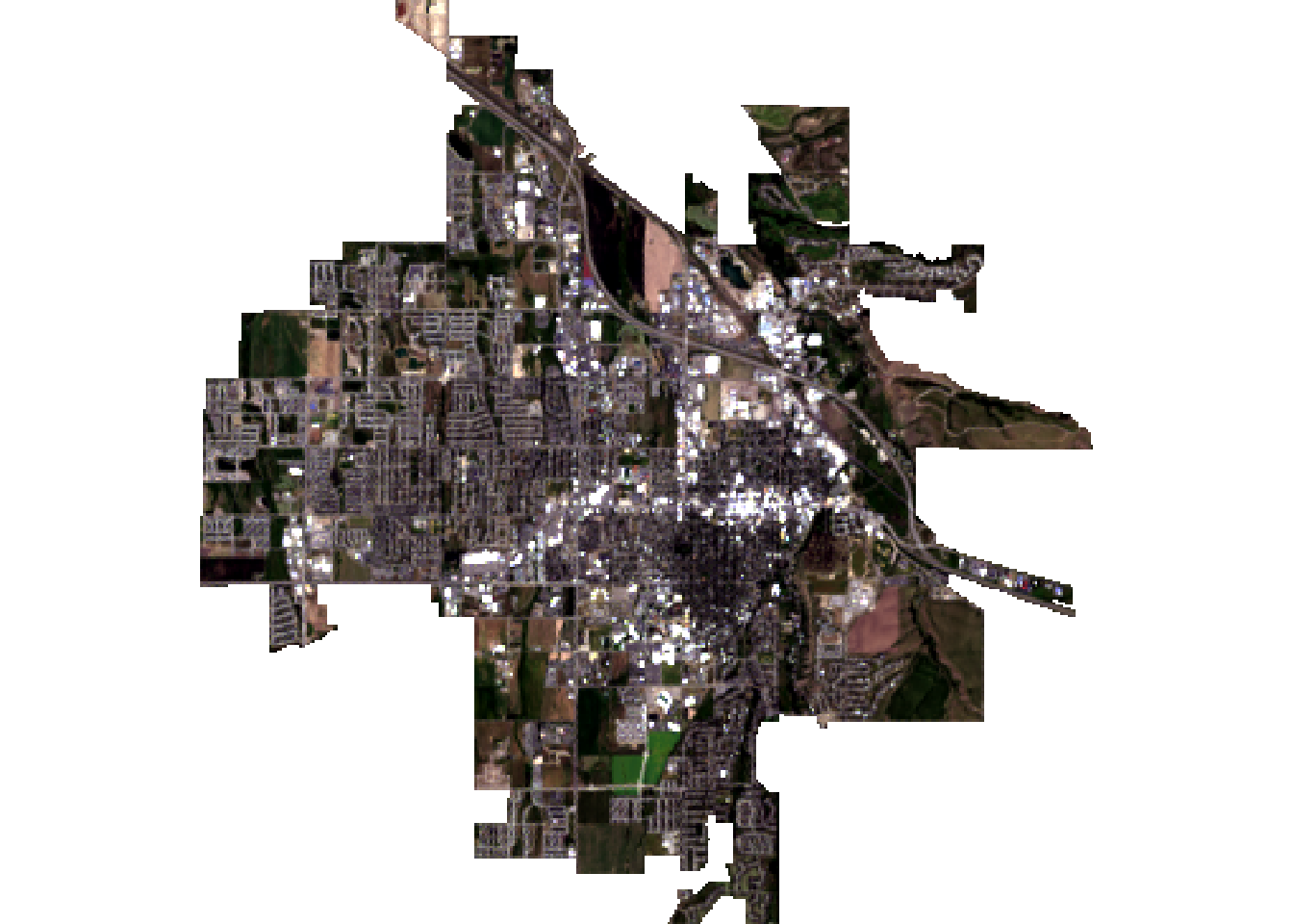
Figure 2: Landsat-8 true color composite cropped to Bozeman city boundaries.

Normalized Difference Vegetation Index

The Normalized Difference Vegetation Index (NDVI) (Kriegler et al. 1969) quantifies vegetation by measuring the difference between near-infrared (which vegetation strongly reflects) and red light (which vegetation absorbs). The NDVI is given by (Akbar 2019):

$$ NDVI = \frac{\rho_{NIR} - \rho_{Red}} {\rho_{NIR} + \rho_{Red}}$$

where \(\rho\) is the surface reflective-values for the near infrared (NIR) and the red (R) spectral bands. Calculations of NDVI for a given pixel always result in a number that ranges from minus one (-1) to plus one (+1).

Akbar et al. (2019) identify suitable NDVI ranges for land cover classes as:

• Water: -0.28 - 0.015
• Built-up: 0.015 - 0.14
• Barren Land: 0.14 - 0.18
• Shrub and Grassland: 0.18 - 0.27
• Sparse Vegetation: 0.27 - 0.36
• Dense Vegetation: 0.36 - 0.74

Healthy vegetation has low red-light reflectance and high near-infrared reflectance that produce high NDVI values. NDVI values near zero and decreasing negative values indicate nonvegetated features, such as barren surfaces (rock and soil), water, snow, ice, and clouds.

Because it is a ratio of two bands, NDVI helps compensate for differences both in illumination within an image due to slope and aspect, and differences between images due things like time of day or season when the images were acquired. Thus, vegetation indices like NDVI make it possible to compare images over time to look for ecologically significant changes. NDVI has seen widespread use in rangeland ecosystems due to its ease of use and relationship to many ecosystem parameters (Landmann and Dubovyk 2014).

Let’s apply a function to calculate the NDVI to the NIR and red bands of the landsat object.

# Create a function that calculates the NDVI
# (NDVI) for each pixel
ndvi <- function(x, y) {
    (x - y) / (x + y)
  }

# Apply function to the NIR and Red bands of 'landsat'
landsatNDVI <- overlay(landsat[[5]], landsat[[4]], fun = ndvi)

# Limit the range of values to be from -1 to 1
landsatNDVI <- reclassify(landsatNDVI, c(-Inf, -1, -1)) # <-1 becomes -1
landsatNDVI <- reclassify(landsatNDVI, c(1, Inf, 1)) # >1 becomes 1

Now, let’s visualize the results.

# Visualise NDVI
par(mar = c(0.2, 0.2, 0.2, 0.2))
plot(
  landsatNDVI, 
  col = rev(terrain.colors(10)), 
  main = NULL, axes = FALSE, box = FALSE
)

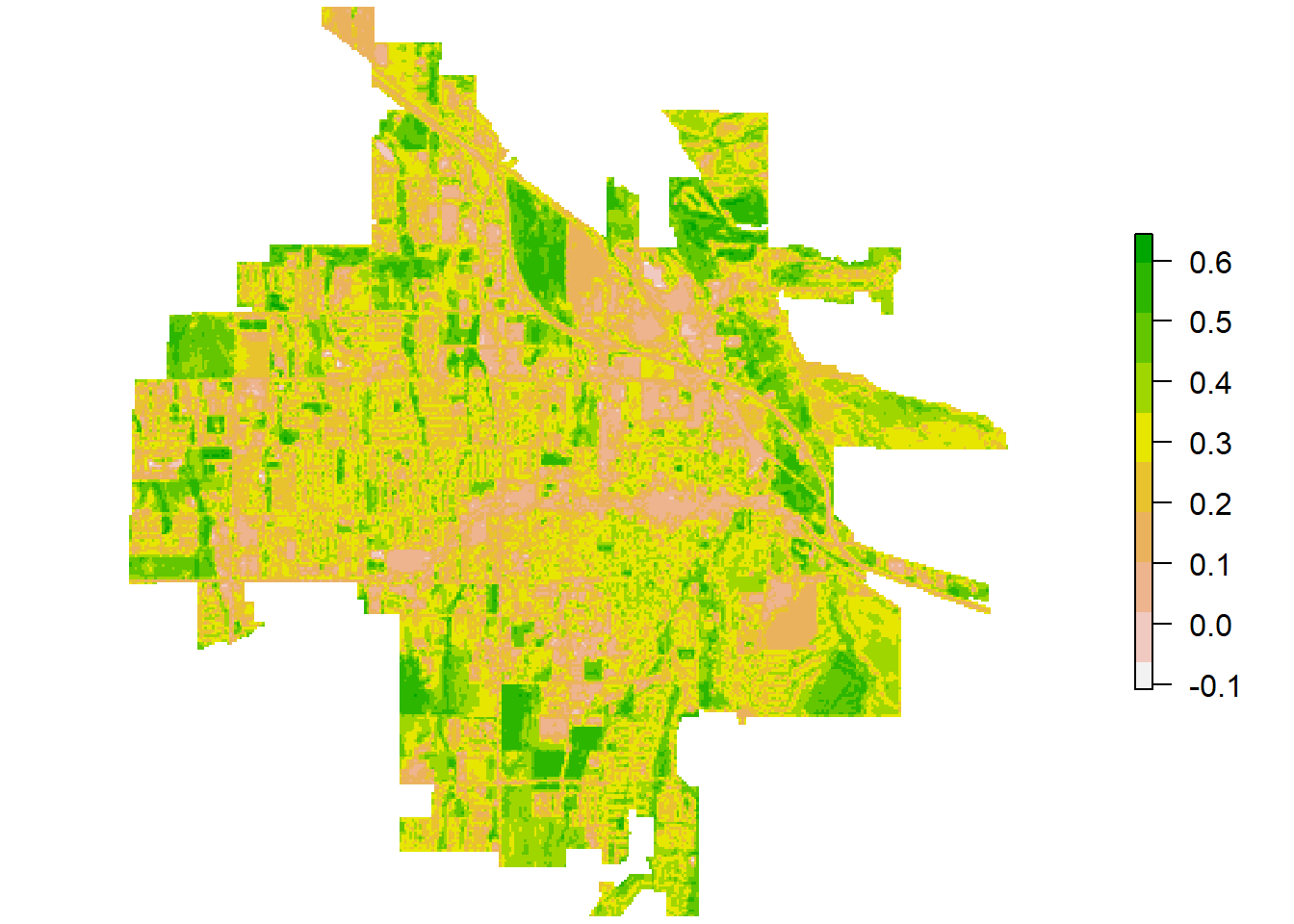
Figure 3: Landsat-8 NDVI for Bozeman.

Let’s create a simple land cover classification in Bozeman using three classes: water, urban, and vegetation.

# Create a matrix to be used as an argument in the 'reclassify()' function
reclass_m <- matrix(
  c(-Inf, 0, 1,   # water
    0, 0.2, 2,    # urban
    0.2, Inf, 3   # veg
  ),
  ncol = 3, byrow = TRUE
)

# Classify land cover using the defined threshold values: 
landsatCover <- reclassify(landsatNDVI, reclass_m)

# Plot the land cover classes
par(mar = c(0.2, 0.2, 0.2, 0.2))
plot(
  landsatCover,
  col = c('blue', 'grey', 'darkgreen'),
  legend = FALSE, axes = FALSE, box = FALSE, main = NULL
)
legend(
  'topright',
  legend = c('Water', 'Urban', 'Vegetation'),
  fill = c('blue', 'grey', 'darkgreen'),
  border = FALSE, bty = 'n'
)

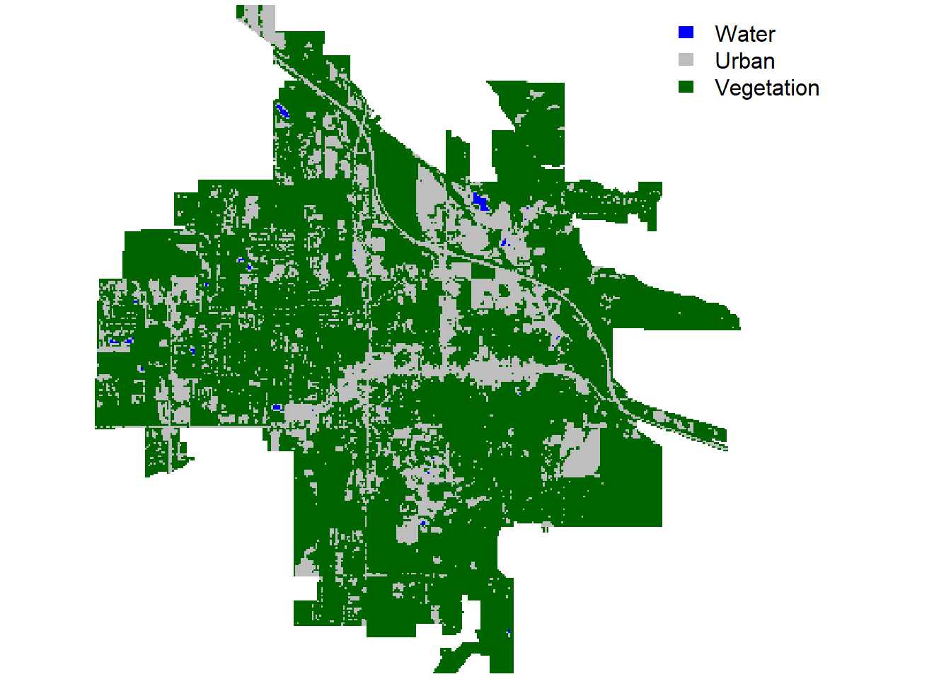
Figure 4: Land cover (mosaic) in Bozeman.

Landscape Metrics

Now, we will calculate landscape metrics for the categorical landscape patterns using the landscapemetrics package. First, we will check the input landscape object. This function extracts basic information about the input landscape, including the type of coordinate reference system (geographic, projected, or NA), units of the coordinate reference system, and the number of classes found in the landscape.

# Load libraries
library(landscapemetrics)
library(landscapetools)

# Check if the raster data is in the right format
check_landscape(landsatCover)

##   layer       crs units   class n_classes OK
## 1     1 projected     m integer         3  v

The landscapemetrics package also can be used to quickly visulaize the landscape.

# Show landscape
show_landscape(landsatCover, discrete = TRUE)

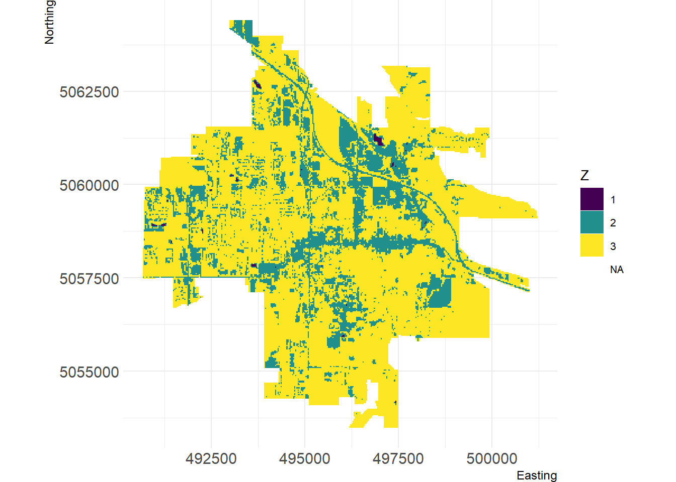
Figure 5: Visualization of Bozeman land cover using landscapemetrics package.

We can create a facet plot of the landscape with the patches labeled using the corresponding patch id, which in this case, corresponds to water (id = 1), urban (id = 2), and vegetation (id = 3).

# Plot landscape
par(mar = c(0.2, 0.2, 0.2, 0.2))
show_patches(landsatCover, class = 'all', labels = FALSE)

## $layer_1

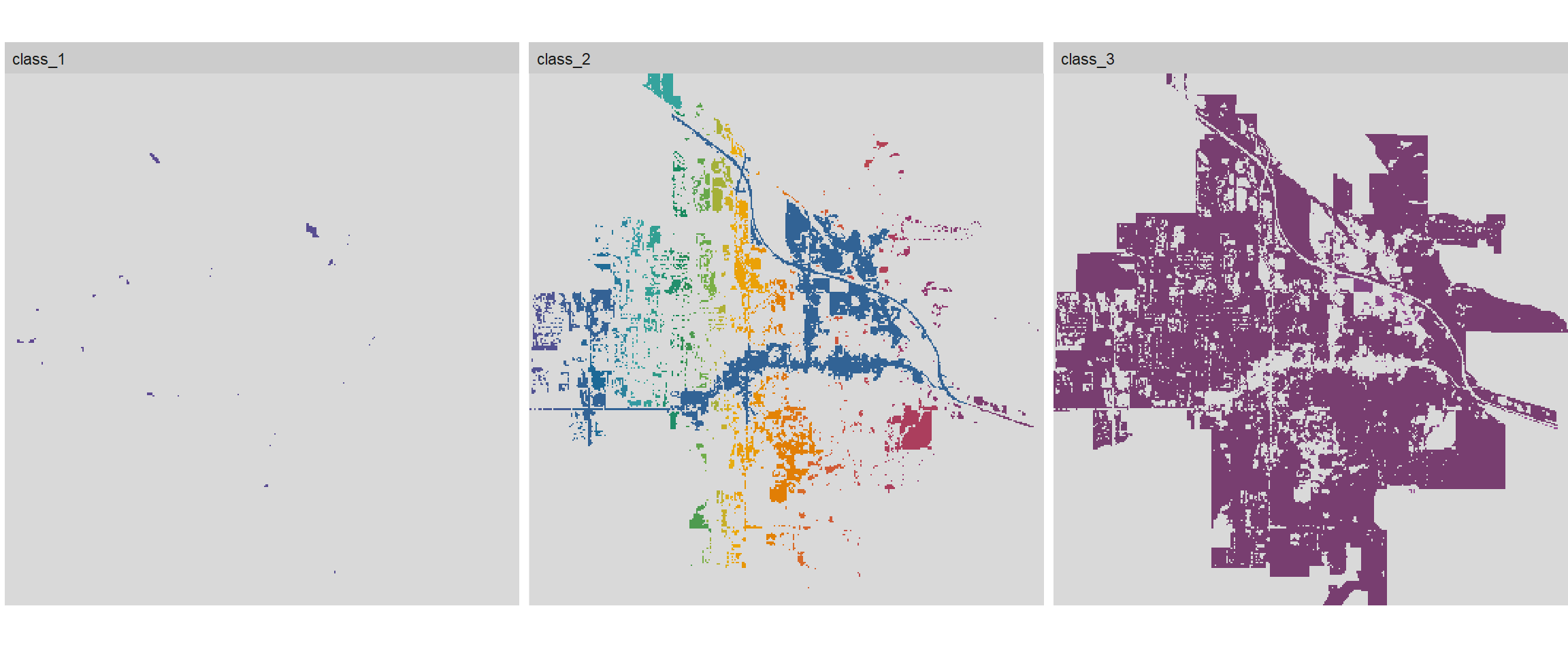
Figure 6: Facet plot of Bozeman land cover with patches.

All functions in landscapemetrics start with lsm_ (for landscapemetrics). The second part of the name specifies the level (p = patch, c = class, or l = landscape). The last part of the function name is the abbreviation of the corresponding metric (e.g., enn for the euclidean nearest-neighbor distance). An example of calculating multiple metrics by name is shown below.

# Calculate multiple metrics by name
calculate_lsm(
  landsatCover, 
  what = c('lsm_l_ta',     # total area of landscape
           'lsm_c_ca',     # total area of each class
           'lsm_c_pland'), # proportional area of each class
  full_name = TRUE
)

## # A tibble: 7 x 9
##   layer level     class    id metric    value name           type  function_name
##   <int> <chr>     <int> <int> <chr>     <dbl> <chr>          <chr> <chr>        
## 1     1 class         1    NA ca       12.2   total (class)~ area~ lsm_c_ca     
## 2     1 class         2    NA ca     1291.    total (class)~ area~ lsm_c_ca     
## 3     1 class         3    NA ca     4433.    total (class)~ area~ lsm_c_ca     
## 4     1 class         1    NA pland     0.213 percentage of~ area~ lsm_c_pland  
## 5     1 class         2    NA pland    22.5   percentage of~ area~ lsm_c_pland  
## 6     1 class         3    NA pland    77.3   percentage of~ area~ lsm_c_pland  
## 7     1 landscape    NA    NA ta     5737.    total area     area~ lsm_l_ta

We can also calculate the diversity of landscape classes as shown below.

# Calculate multiple metrics by level and type
calculate_lsm(
  landsatCover, 
  level = 'landscape',
  type = 'diversity metric',
  full_name = TRUE
)

## # A tibble: 9 x 9
##   layer level     class    id metric   value name            type  function_name
##   <int> <chr>     <int> <int> <chr>    <dbl> <chr>           <chr> <chr>        
## 1     1 landscape    NA    NA msidi   0.434  modified simps~ dive~ lsm_l_msidi  
## 2     1 landscape    NA    NA msiei   0.395  modified simps~ dive~ lsm_l_msiei  
## 3     1 landscape    NA    NA pr      3      patch richness  dive~ lsm_l_pr     
## 4     1 landscape    NA    NA prd     0.0523 patch richness~ dive~ lsm_l_prd    
## 5     1 landscape    NA    NA rpr    NA      relative patch~ dive~ lsm_l_rpr    
## 6     1 landscape    NA    NA shdi    0.548  shannon's dive~ dive~ lsm_l_shdi   
## 7     1 landscape    NA    NA shei    0.499  shannon's even~ dive~ lsm_l_shei   
## 8     1 landscape    NA    NA sidi    0.352  simpson's dive~ dive~ lsm_l_sidi   
## 9     1 landscape    NA    NA siei    0.528  simspon's even~ dive~ lsm_l_siei

Moab, Utah

Similar to the landscape pattern analysis conducted for Bozeman, we will quickly analyze the landscape in Moab, Utah using the Landsat-8 scene on June 30, 2020 with a 30 m resolution for the RGB, NIR, and SWIR bands. The Landsat-8 NDVI for Moab shown below indicates a landscape in Moab mainly composed of barren land and sparse vegetation. To account for this difference, we can create a more detailed land cover classification using five classes: water, urban, barren land, sparse vegetation, and dense vegetation.

## Reading layer `Moab' from data source 
##   `C:\Users\cholbert\mywebsite\content\blog\landscape_pattern_analysis\data\shapefiles\Moab.shp' 
##   using driver `ESRI Shapefile'
## Simple feature collection with 1 feature and 8 fields
## Geometry type: POLYGON
## Dimension:     XY
## Bounding box:  xmin: 623741.7 ymin: 4266336 xmax: 629398.1 ymax: 4273712
## Projected CRS: NAD83 / UTM zone 12N

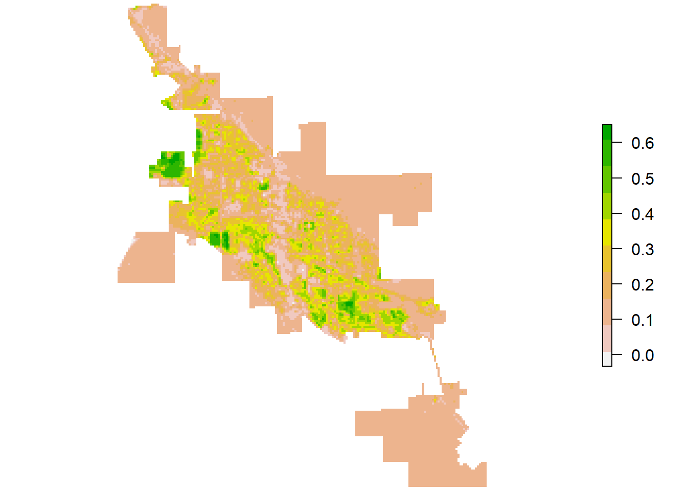
Figure 7: Landsat-8 NDVI for Moab.

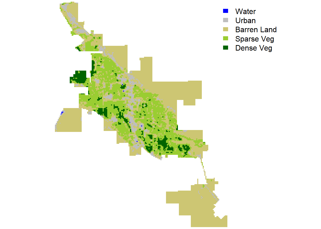
Figure 8: Land cover (mosaic) in Moab.

# Show landscape
show_landscape(landsatCover, discrete = TRUE)

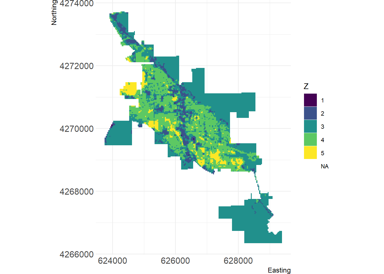
Figure 9: Visualization of Moab land cover using landscapemetrics package.

Conclusion

Multispectral remotely sensed imagery are a rich resource for landscape pattern analysis. The workflow presented in this factsheet can be used as a guide when using R for image processing to understand categorical landscape patterns. The use of NDVI facilitates remote sensing applications in part because it correlates with the status of a broad array of vegetation properties. However, the effective use of NDVI depends on the quality of multispectral data and the interpretation of NDVI values. Although this analysis suggests that patterns can be characterized by a few simple metrics, there is seldom a one-to-one relationship between metric values and pattern. The format and scale of the data can have a significant influence on the value of many metrics. The importance of fully understanding each landscape metric before it is selected for interpretation cannot be over emphasized.

References

Akbar, T.A., Q.K. Hassan, S. Ishaq, M. Batool, H.J. Butt, and H. Jabbar. 2019. Investigative spatial distribution and modelling of existing and future urban land changes and its impact on urbanization and economy. Remote Sens, 11:1-15.

Chuvieco, E. 1999. Measuring changes in landscape pattern from satellite images: short-term effects of fire on spatial diversity. International Journal of Remote Sensing, 20:2331-2346.

Foley, J.A., R. DeFries, G.P. Asner, C. Barford, G. Bonan, S.R. Carpenter, F.S. Chapin, M.T. Coe1, G.C. Daily, H.K. Gibbs, J.H. Helkowski, T. Holloway, E. A. Howard, C.J. Kucharik, C. Monfreda, J.A. Patz, I.C. Prentice, N. Ramankutty, and P.K. Snyder. 2005. Global consequences of land use. Science, 309:570-574.

Hesselbarth, M.H.K., M. Sciaini, K.A. With, K. Wiegand, and J. Nowosad. 2019. landscapemetrics: an open-source R tool to calculate landscape metrics. Ecography, 42:1648-1657 (ver. 0).

Kriegler F.J., W.A. Malila, R.F. Nalepka, and W. Richardson. 1969. Preprocessing transformations and their effect on multispectral recognition. Remote Sens Environ, VI:97-132.

Landmann, T. and O. Dubovyk. 2014. Spatial analysis of human-induced vegetation productivity decline over eastern Africa using a decade (2001-2011) of medium resolution MODIS time-series data. Int. J. Appl. Earth Observ. Geoinformation, 33:76-82.

McGarigal, K., and B.J. Marks. 1995. FRAGSTATS: Spatial Pattern Analysis Program for Quantifying Landscape Structure. USDA Forest Service General Technical Report PNW-351, Corvallis.

McGarigal, K., S.A. Cushman, E. Ene. 2012. FRAGSTATS v4: Spatial Pattern Analysis Program for Categorical and Continuous Maps. Computer software program produced by the authors at the University of Massachusetts, Amherst. Available at the following website: http://www.umass.edu/landeco/research/fragstats/fragstats.html

R Core Team. 2020. R: A language and environment for statistical computing. R Foundation for Statistical Computing, Vienna, Austria. URL https://www.R-project.org/.

United States Geological Survey (USGS). 2021. Landsat Missions. https://www.usgs.gov/core-science-systems/nli/landsat/landsat-8?qt-science_support_page_related_con=0#qt-science_support_page_related_con.

Young, N.E., R.S. Anderson, S.M.Chignell, A.G. Vorster, R. Lawrence, and P.H. Evangelista. 2017. A survival guide to Landsat preprocessing. Ecology, 98:920-932.