Lognormal Kriging and Bias-Corrected Back-Transformation
By Charles Holbert
August 15, 2024
Introduction
Kriging does not assume any specific distribution for the variable being estimated; instead, it relies on the assumption of spatial stationarity. Because kriging involves computing a weighted average of nearby values, non-symmetric distributions, such as positively-skewed distributions common in earth sciences, can pose challenges. The presence of a few high values increase the variance of the data set and make variogram calculation and kriging estimation difficult, potentially leading to over-prediction and difficulties in modeling.
To address this issue, non-symmetric distributions are often transformed before performing variogram analysis and kriging. A common transformation for highly-skewed unimodal distributions is the natural logarithm, which can help normalize the distribution and stabilize variances, resulting in what is known as lognormal kriging. However, a challenge arises when wanting to back-transform estimates and their variances from the transformed domain to the original scale of the data.
In this post we will examine lognormal kriging and the mathematical formulations derived to back-transform the prediction and prediction variance to the original measurement scale. Variogram modeling and kriging are performed using the gstat library (Pebesma 2004; Graler et al. 2016) within the R language for statistical computing and data visualization (R Core Team 2024).
Background
In lognormal kriging, the data undergo transformation into their natural logarithms, which act as a sample from a random variable \(Y(\mathbf{x}) = logZ(\mathbf{x})\) assumed to have second-order stationarity. The variogram of \(Y(\mathbf{x})\) is calculated and modeled, and this is subsequently utilized alongside the transformed data to estimate Y at the target locations using either ordinary kriging (OK) or simple kriging (SK). Estimates at the unsampled locations are in the logarithmic domain, \(\hat{Y}(\mathbf{x}_0)\) rather than \(\hat{Z}(\mathbf{x}_0)\), and need to be back-transformed into the original scale of measurement.
To obtain the kriged estimate, we typically require the back-transformed estimate. We cannot reverse the transformation through simple exponentiation because the estimate is a weighted sum of sample values derived from log-transformed data, while the sum of logarithms corresponds to a product. As a result, the weighting approach differs from what it would be if we had used the original (untransformed) values. Additionally, exponentiating a symmetric (Gaussian) prediction variance leads to right-skewed results. The correct back-transformation was derived by Journel (1980) and is presented in Webster and Oliver (2007). Journel and Huijbregts (1978) highlight that back-transforming data from lognormality can be sensitive to deviations, which may lead to biased estimates of Z. However, lognormal kriging is commonly employed to symmetrize positively-skewed distributions, provided there are no zero data points, and it is generally effective for this purpose.
In the case of Simple Kriging (SK), where the mean is known, it is possible to back-transform both the estimates and their variances. If we denote the kriged estimate of the natural logarithm at \(\mathbf{x}_0\) as \(\hat{Y}(\mathbf{x}_0)\) and its variance as \(\sigma^{2}(\mathbf{x}_0)\), the formula for back-transformation of the estimates are, for simple kriging:
$$\hat{Z}_{SK}(\mathbf{x}_0) = exp[\hat{Y}_{SK}(\mathbf{x}_0) + \sigma^2_{SK}(\mathbf{x}_0)/2]$$
The estimates are always increased because the prediction variance \(\sigma^2_{SK}\) is positive. This increase is a result of the skewed distribution of the back-transformed prediction variance.
The back-transformed prediction variance of \(Z(\mathbf{x}_0)\) for SK is given by:
$$var_{SK}[\hat{Z}(\mathbf{x}_0)] = \mu^2_Z exp(\sigma^2_{SK})[1 - exp{(-\sigma^2_{SK}(\mathbf{x}_0)/2})]$$
where \(\mu_Z\) is the expected value of \(Z(\mathbf{x}_0)\). This in turn is back-transformed from the best linear unbiased estimator (BLUE) prediction of the log-transformed spatial mean \(\mu_Y\) as:
$$\mu_Z = exp[\mu_Y + \sigma^2(\mu_Y)/2]$$
where \(\mu_Y\) is the BLUE prediction of the spatial mean and \(\sigma^2(\mu_Y)\) is its prediction variance. This is the same formula for back-transformation of a log-transformed variable used above for the SK predictions.
In the case of OK, where the true spatial mean is not known, only the predicted value can be derived. The predicted values of target variable Z can be derived from its log-transform Y = log(Z) at prediction location \(\mathbf{x}_0\) using the following formula:
$$\hat{Z}_{OK}(\mathbf{x}_0) = exp[\hat{Y}_{OK}(\mathbf{x}_0) + \sigma^2_{OK}(\mathbf{x}_0)/2 - \psi_{OK}]$$
where \(\psi_{OK}\) is the LaGrange multiplier in the solution of the OK system. The LaGrange multiplier is not required when back-transforming the estimates and their variances for SK.
Data
The meuse data set, sourced from Pebesma (2022) and included in the sp library, contains measurements of four heavy metals (in parts-per-million) sampled from the topsoil of a floodplain near the village Stein in the Netherlands. The samples are taken from an area approximately 15m by 15m, along with various covariates. Additionally, the sp library features the meuse.grid data frame, which represents a 40m x 40m grid covering the Meuse study area. The coordinates used are in the Rijksdriehoek (RDH) format, which is specific to Dutch topographical mapping.
For this example, we will use the zinc topsoil concentration data.
# Load libraries
library(dplyr)
library(sp)
library(gstat)
library(lattice)

# Load functions
source('functions/univariate_plots.R')

# Load data
data(meuse)
data(meuse.grid)

# Prep data
dat <- meuse %>%
  dplyr::select(x, y, zinc) %>%
  rename(Zn = zinc) %>%
  mutate(lZn = log(Zn)) %>%
  data.frame()
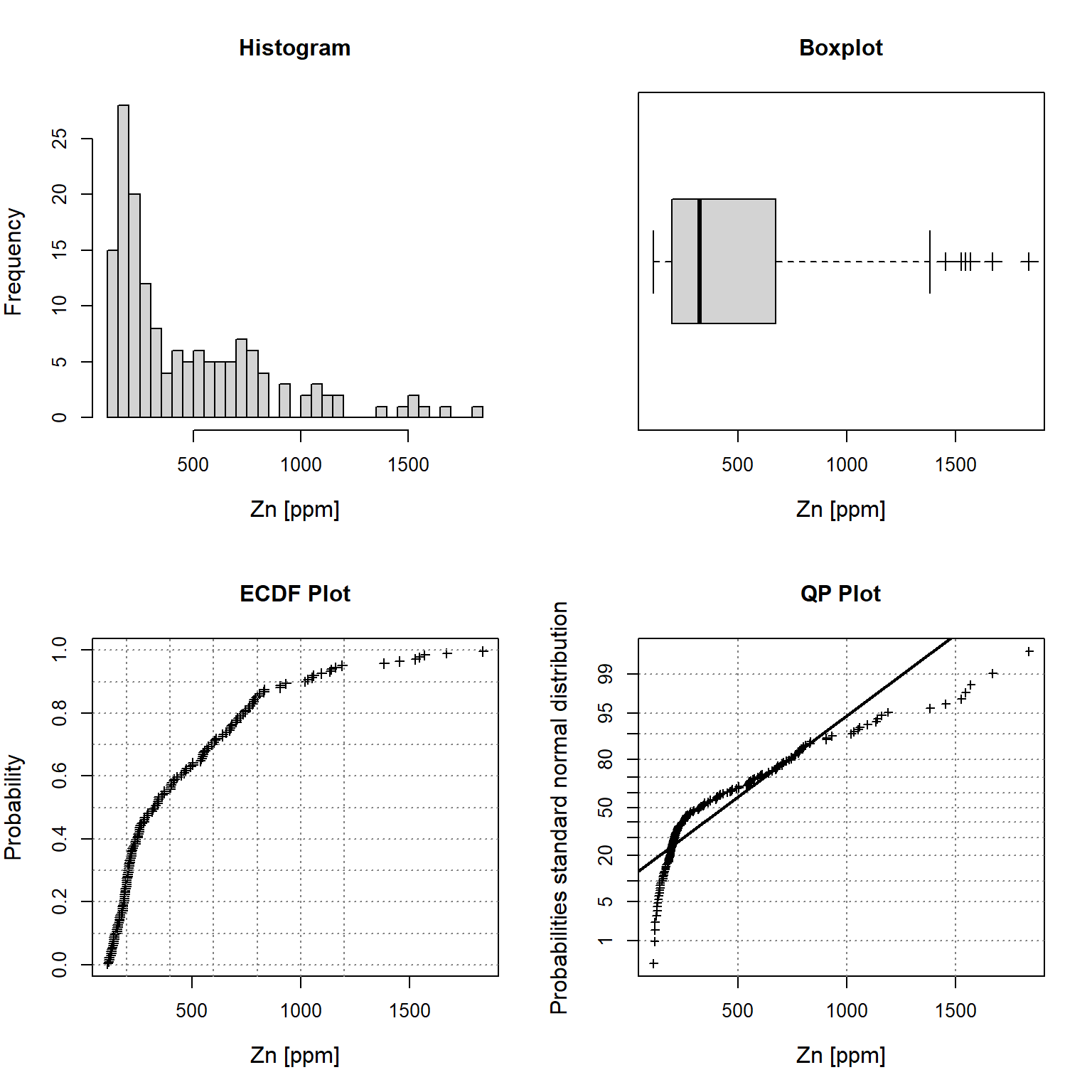
Let’s inspect univariate plots of the zinc topsoil concentrations. These plots can be used to understand the characteristics of the observed data, including the data distribution; the median, skewness, and tailedness of the distribution; and to identify data outliers. The plots include a histogram in the upper left window, an empirical cumulative density function (ECDF) plot in the lower left window, a box plot in the upper right window, and a cumulative probability (CP) plot in the lower right window.
# Plot univariate plots of raw data
univPlots(
  x = dat$Zn,
  xlabel = 'Zn [ppm]'
)
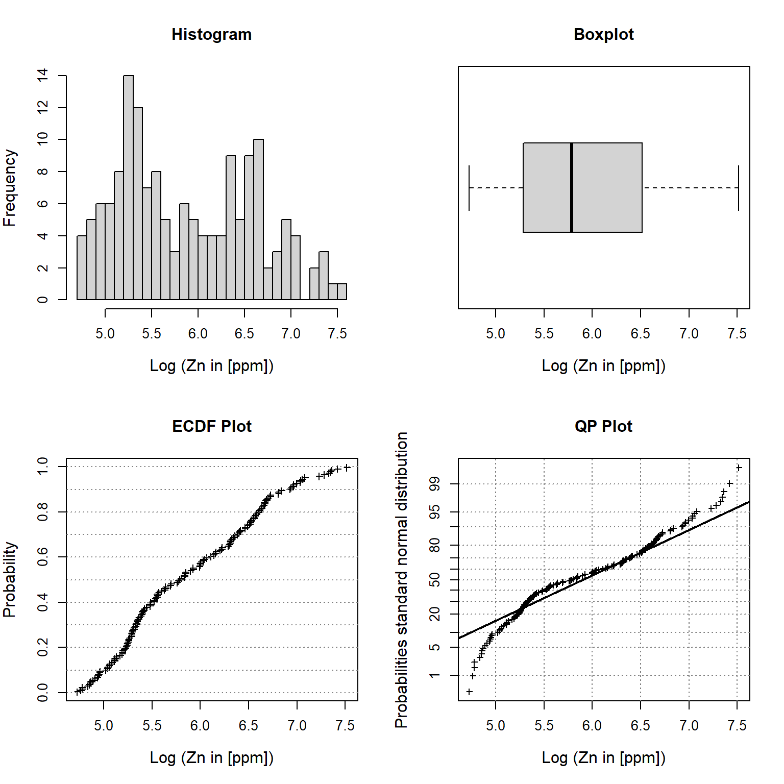
Let’s inspect univariate plots of the natural log transformed zinc topsoil concentrations.
# Plot univariate plots of log transformed data
univPlots(
  x = dat$lZn,
  xlabel = 'Log (Zn in [ppm])'
)
Variograms
Let’s compute and model the local spatial dependence for the original (untransformed) variable and the natural log transformed variable.
Original Data
First, let’s compute the empirical variogram of the untransformed zinc topsoil concentrations and then fit an omnidirectional spherical variogram model to the data.
# Make data geospatial object
coordinates(dat) = ~x+y

# Calculate experimental variogram for Zn
v <- variogram(Zn ~ 1, data = dat)

# Fit omnidirectional spherical variogram model
vm <- fit.variogram(
  v,
  vgm(150000, 'Sph', 800, 0)
)

# Create table of model variogram parameters
knitr::kable(vm[, 1:3]) %>%
  kableExtra::kable_classic_2(
    full_width = F, position = 'center', html_font = 'Cambria'
  )
| model | psill | range |
|---|---|---|
| Nug | 24796.16 | 0.000 |
| Sph | 134741.79 | 830.836 |
# Plot experimental and model variogram
plot(
  v, vm,
  main = 'Variogram Original Zinc Data',
  xlab = 'Distance (m)', ylab = 'Semivariance',
  pch = 16, cex = 1
)
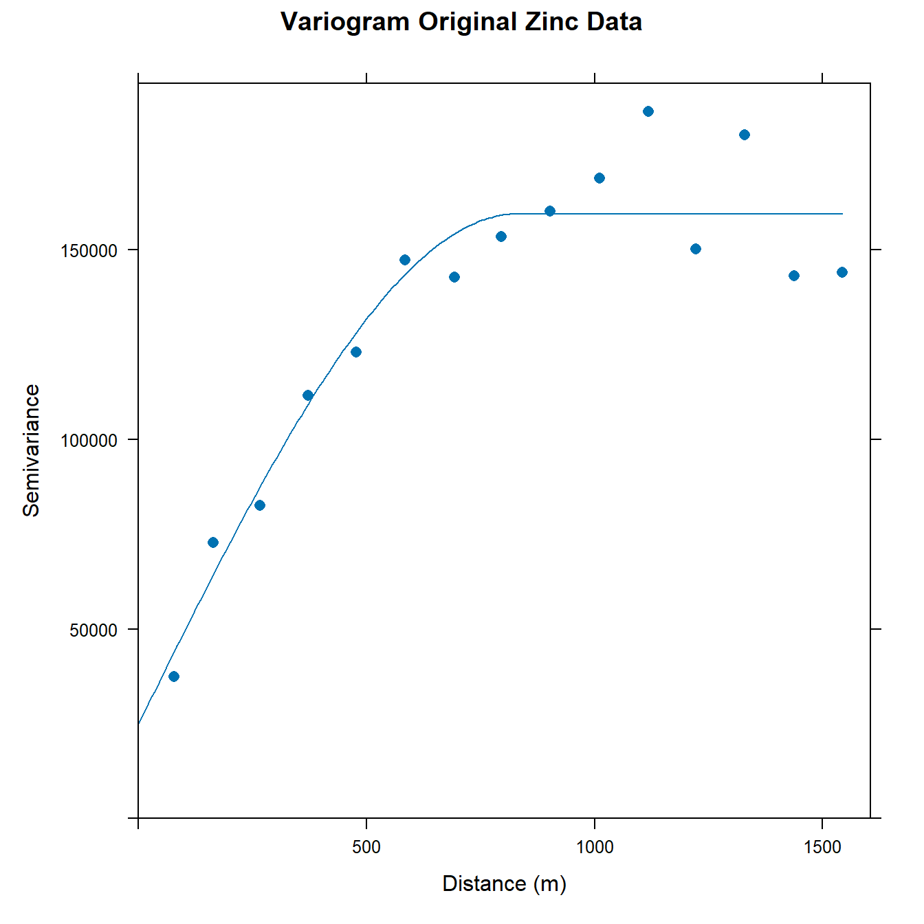
We can compute the proportion of variance explained for the untransformed variable, which is given by the structural sill divided by the total sill.
vm[2, 'psill']/sum(vm[, 'psill'])
## [1] 0.8445752
Transformed Data
Now, let’s compute the empirical variogram of the natural log transformed zinc topsoil concentrations and then fit an omnidirectional spherical variogram model to the transformed data.
# Calculate experimental variogram for log(Zn)
v.log <- variogram(lZn ~ 1, data = dat)

# Fit omnidirectional spherical variogram model
vm.log <- fit.variogram(
  v.log,
  vgm(0.6, 'Sph', 800, 0)
)

# Create table of model variogram parameters
knitr::kable(vm.log[, 1:3]) %>%
  kableExtra::kable_classic_2(
    full_width = F, position = 'center', html_font = 'Cambria'
  )
| model | psill | range |
|---|---|---|
| Nug | 0.0506561 | 0.0000 |
| Sph | 0.5906014 | 896.9743 |
# Plot experimental and model variogram
plot(
  v.log, vm.log,
  main = 'Variogram Transformed Zinc Data',
  xlab = 'Distance (m)', ylab = 'Semivariance',
  pch = 16, cex = 1
)
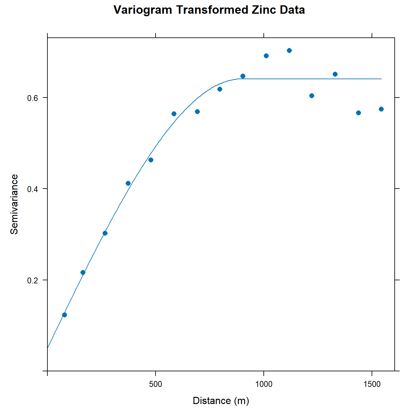
Let’s compute the proportion of variance explained for the transformed variable.
vm.log[2, 'psill']/sum(vm.log[, 'psill'])
## [1] 0.9210051
Ordinary Kriging
Let’s use our variogram model for the original (untransformed) data to estimate zinc concentrations at unsampled locations across the meuse grid using ordinary kriging. First, let’s convert the meuse.grid data frame to a spatial pixels data frame, which will be used to store the kriging estimates.
# Convert meuse grid to a spatial points data frame
coordinates(meuse.grid) <- ~ x + y

# Convert meuse grid to a spatial pixels data frame
gridded(meuse.grid) = TRUE

# Ordinary kriging of raw data
k <- krige(
  Zn ~ 1, dat,
  meuse.grid,
  model = vm
)
## [using ordinary kriging]
# Store predictions in meuse.grid
meuse.grid$Zn.pred <- k@data$var1.pred
Let’s now utilize our variogram model for the transformed data to estimate zinc concentrations at unsampled locations across the meuse grid through ordinary kriging. In a straightforward approach, we’ll back-transform the log estimates by applying the reverse of the transformation (exponentiation). However, it’s important to note that this method is not accurate because the log estimate represents a weighted sum of the sample values of log(Zn), and the sum of logarithms corresponds to a product. Consequently, the weighting scheme for the log-transformed data differs from that of the original (untransformed) values. Nonetheless, we can still compare these biased back-transformed estimates with those obtained using the correct back-transformation method.
# Ordinary kriging of raw data
k <- krige(
  lZn ~ 1, dat,
  meuse.grid,
  model = vm.log
)
## [using ordinary kriging]
# Exponentiate log-transformed predictions and store in meuse.grid
meuse.grid$lZn.pred <- exp(k@data$var1.pred)
Bias-Corrected Back-Transformation
The gstat library does not employ minimization with LaGrange multipliers to solve the kriging system, so the previously mentioned back-transformation formula for OK cannot be utilized. Instead, gstat adopts a regression method for kriging using the following steps:
-
First, gstat determines the spatial mean (or regional trend for universal kriging) using Generalized Least Squares (GLS). This process necessitates an understanding of the covariance structure, which is identified through variogram modeling, to account for the spatial correlation in the observations.
-
Next, gstat performs SK on the residuals derived from the calculated mean (or trend).
-
The final prediction at a given point is obtained by adding the spatial mean (or trend) to the predicted residual for that specific point.
Both the computation of the spatial mean (or trend) and SK give a standard error of prediction, which can be added for a final standard error.
In gstat, if you set the optional BLUE argument of the krige method to TRUE, it will return the BLUE prediction of the parameter. By default, this argument is set to FALSE, which means it returns the best linear unbiased predictor (BLUP) of the point. Typically, the BLUP is the desired output, as it represents the predicted value at that specific location. On the other hand, the BLUE represents the spatial mean, or the expected value, without considering the influence of nearby points.
Unfortunately, the krige() function in gstat does not provide an option to obtain only the BLUE. Instead, we must first create a new gstat object using the gstat() function, indicating that it is a new object by passing NULL as the first argument. This new object will contain all the information about the variable, including the data, the locations, and the variogram model.
g <- gstat(
  NULL, id = "lZn", form = lZn ~ 1,
  data = dat, model = vm.log
)
We can now utilize the predict() function in gstat. Because all locations will yield the same BLUE for OK due to the absence of a trend, it is enough to make a prediction at just one location. Let’s perform the prediction for the first point in the grid. We can extract this point using the standard “[” operator, ensuring we maintain the entire grid topology by including the optional drop=FALSE argument. Next, we will convert this into a single spatial point using the SpatialPoints() function, which can then be employed as new data for prediction.
dat.one <- SpatialPoints(meuse.grid[1, drop = FALSE])
k.blue <- predict(g, newdata = dat.one, BLUE = T)
## [generalized least squares trend estimation]
k.blue$lZn.pred
## [1] 6.053536
k.blue$lZn.var
## [1] 0.03981609
# Back-transform expected value to original units
(Zn.blue <- exp(k.blue$lZn.pred + k.blue$lZn.var/2))
## [1] 434.1732
Next we compute the residuals at the observation points and add them to the data:
# Compute residuals
dat$lZn.res <- dat$lZn - k.blue$lZn.pred
summary(dat$lZn.res)
##    Min. 1st Qu.  Median    Mean 3rd Qu.    Max.
## -1.3261 -0.7653 -0.2666 -0.1678  0.4604  1.4634
Now, we utilize SK for predictions, assuming a known (spatial) mean of zero. Note that SK will be employed by gstat if the optional beta parameter is provided in the call to the krige() function.
# Finally, use SK to predict, with the known (spatial) mean of zero
k.res.sk <- krige(
  lZn.res ~ 1, dat,
  newdata = meuse.grid,
  model = vm.log, beta = 0
)
## [using simple kriging]
summary(k.res.sk)
## Object of class SpatialPixelsDataFrame
## Coordinates:
##      min    max
## x 178440 181560
## y 329600 333760
## Is projected: NA
## proj4string : [NA]
## Number of points: 3103
## Grid attributes:
##   cellcentre.offset cellsize cells.dim
## x            178460       40        78
## y            329620       40       104
## Data attributes:
##    var1.pred          var1.var
##  Min.   :-1.2770   Min.   :0.08549
##  1st Qu.:-0.8159   1st Qu.:0.13728
##  Median :-0.4806   Median :0.16215
##  Mean   :-0.3463   Mean   :0.18485
##  3rd Qu.: 0.1182   3rd Qu.:0.21128
##  Max.   : 1.3865   Max.   :0.48872
Finally, we back-transform the residuals and the prediction variances to the original units of measurement:
# Back transform residuals
k.res.sk$res.pred <- exp(k.res.sk$var1.pred + k.res.sk$var1.var/2)
summary(k.res.sk$res.pred)
##    Min. 1st Qu.  Median    Mean 3rd Qu.    Max.
##  0.2967  0.4820  0.6708  0.9306  1.2593  4.3045
# Back transform variance
mu.Z <- exp(k.blue$lZn.var/2)
k.res.sk$res.var <- mu.Z^2 * exp(k.res.sk$var1.var) * (1 - exp(-k.res.sk$var1.var)/2)
summary(k.res.sk$res.var)
##    Min. 1st Qu.  Median    Mean 3rd Qu.    Max.
##  0.6132  0.6734  0.7035  0.7348  0.7651  1.1761
To obtain the BLUP in its original units, we multiply the back-transformed spatial mean by the back-transformed residuals. It’s important to note that the variance remains consistent whether considering the residuals or the original values.
meuse.grid$BTZn.pred <- Zn.blue * k.res.sk$res.pred
summary(meuse.grid$BTZn.pred)
##    Min. 1st Qu.  Median    Mean 3rd Qu.    Max.
##   128.8   209.3   291.3   404.1   546.7  1868.9
Results
Having obtained kriging predictions for zinc concentrations in the topsoil along the Meuse River using all our variogram models, let’s examine and compare the sample statistics of the original (untransformed) data with those of the kriging models.
# Compare sample statistics
cdat <- cbind(
  data.frame(unclass(summary(dat@data$Zn))),
  data.frame(unclass(summary(meuse.grid@data$Zn.pred))),
  data.frame(unclass(summary(meuse.grid@data$lZn.pred))),
  data.frame(unclass(summary(meuse.grid@data$BTZn.pred)))
)
names(cdat) <- c('Raw.Data', 'OK', 'OK.Exp', 'OK.BT')

# Create table of model variogram parameters
knitr::kable(round(cdat, 0)) %>%
  kableExtra::kable_classic_2(
    full_width = F, position = 'center', html_font = 'Cambria'
  )
| Raw.Data | OK | OK.Exp | OK.BT | |
|---|---|---|---|---|
| Min. | 113 | 46 | 119 | 129 |
| 1st Qu. | 198 | 211 | 188 | 209 |
| Median | 326 | 316 | 263 | 291 |
| Mean | 470 | 409 | 362 | 404 |
| 3rd Qu. | 674 | 556 | 479 | 547 |
| Max. | 1839 | 1598 | 1703 | 1869 |
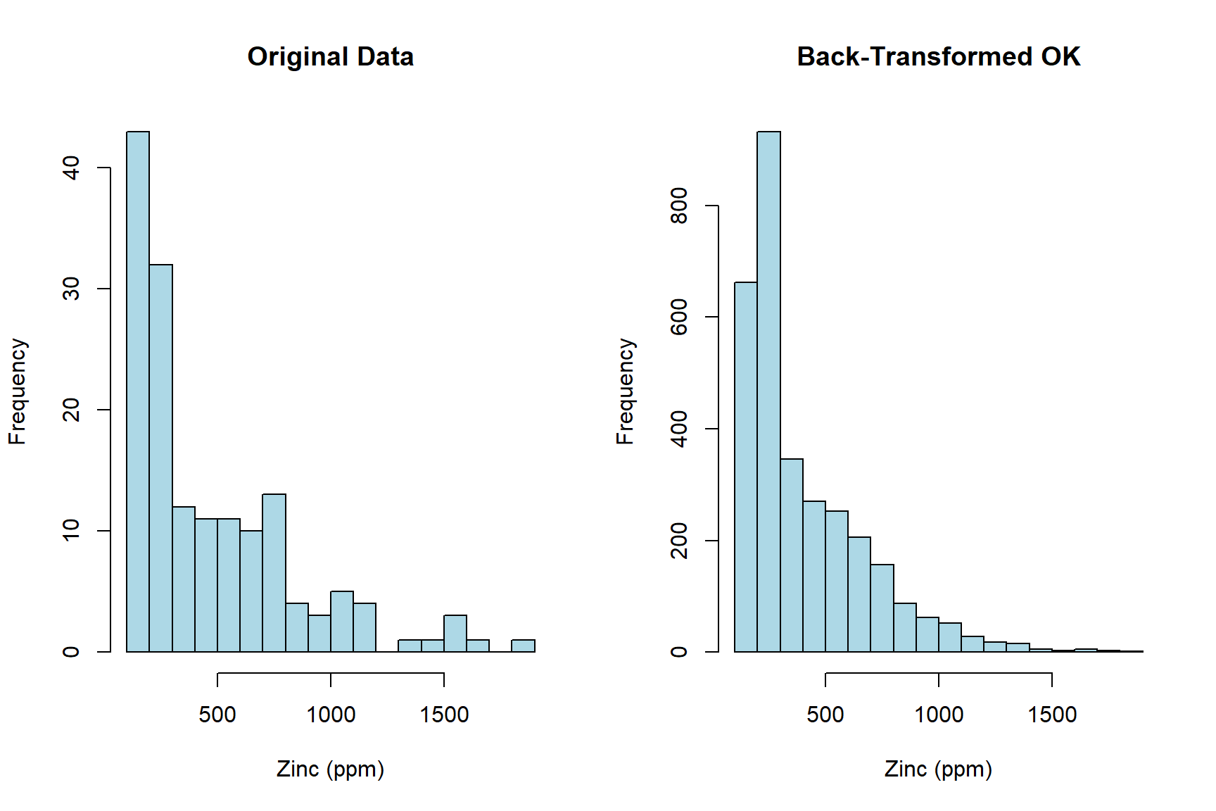
Accurate inferences about a population depend on how closely estimates match sample data. Given that we lack information about the population from which the sample is drawn, the ideal approach is to keep the estimates of the spatial phenomenon as close as possible to the sample statistics. In this context, the bias-corrected back-transformed OK results provides an estimated distribution that generally aligns with the sample statistics. In comparison, the other methods perform poorly against the sample statistics.
Let’s compare histograms of the original (untransformed) data and the back-transformed lognormal OK estimates.
# Display histogram of raw data and back-transformed OK estimates
par(mfrow = c(1, 2))
hist(
  dat@data$Zn,
  breaks = 20, col = 'lightblue',
  main = 'Original Data',
  xlab = 'Zinc (ppm)'
)
hist(
  meuse.grid@data$BTZn.pred,
  breaks = 20, col = 'lightblue',
  main = 'Back-Transformed OK',
  xlab = 'Zinc (ppm)'
)
par(mfrow = c(1, 1))
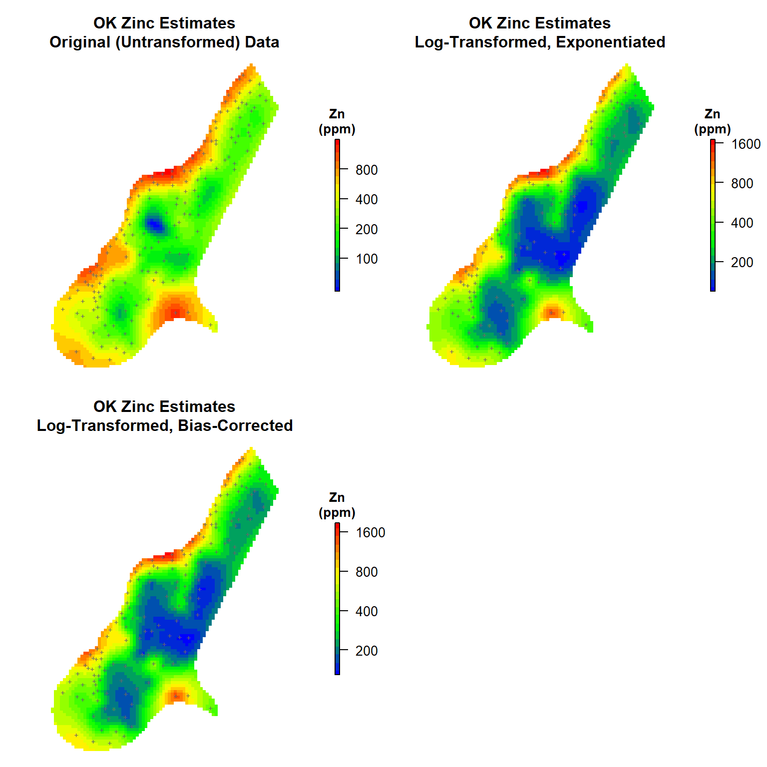
Let’s generate contour maps to illustrate the variations between the OK estimates and those derived from the exponentiated and bias-corrected lognormal OK estimates.
# Load library
library(raster)

# Create color-scale for plot
leg <- c(
  "#0000ff", "#0028d7", "#0050af", "#007986", "#00a15e",
  "#00ca35", "#00f20d", "#1aff00", "#43ff00", "#6bff00",
  "#94ff00", "#bcff00", "#e5ff00", "#fff200", "#ffca00",
  "#ffa100", "#ff7900", "#ff5000", "#ff2800", "#ff0000"
)

# Create breaks for legend
axis.ls <- list(
  at = log10(c(100, 200, 400, 800, 1600)),
  labels = c(100, 200, 400, 800, 1600)
)

# Function to create plots
get_plot <- function(d, mtitle) {
  plot(
    log10(raster(d)),
    col = leg,
    main = mtitle,
    axes = FALSE,
    box = FALSE,
    axis.args = axis.ls,
    legend.args = list(
      text = 'Zn\n(ppm)',
      side = 3, font = 2, line = 0.2, cex = 0.8
    )
  )
  points(coordinates(dat), pch = "+", cex = 0.6, col = 'grey40')
}

# Create plots
par(mfrow = c(2, 2), oma = c(0, 0, 0, 1), mar = c(1, 1, 4, 3))

# Map #1
get_plot(
  d = meuse.grid['Zn.pred'],
  mtitle = 'OK Zinc Estimates\nOriginal (Untransformed) Data'
)

# Map # 2
get_plot(
  d = meuse.grid['lZn.pred'],
  mtitle = 'OK Zinc Estimates\nLog-Transformed, Exponentiated'
)

# Map # 3
get_plot(
  d = meuse.grid['BTZn.pred'],
  mtitle = 'OK Zinc Estimates\nLog-Transformed, Bias-Corrected'
)
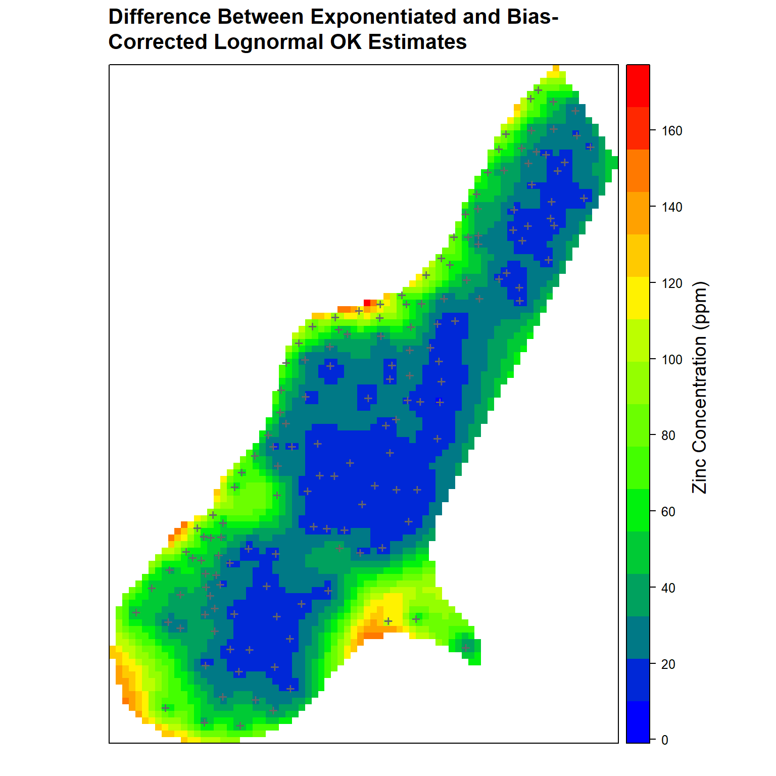
In conclusion, let’s create a contour map that highlights the differences between the exponentiated estimates and the bias-corrected lognormal OK estimates.
# Load library
library(grid)

# Get difference between exponentiated and bias-corrected OK estimates
meuse.grid$Diff <- meuse.grid$BTZn.pred - meuse.grid$lZn.pred

# Re-define default color scheme
old_theme <- get_col_regions()
new_theme <- set_col_regions(leg)

# Set main title settings
my.settings <- list(
  par.main.text = list(
    fontsize = 13,
    just = 'left',
    x = grid::unit(6, 'mm')
  )
)

# Create plot comparing differences between exponentiated and bias-corrected
# OK estimates
spplot(
  meuse.grid['Diff'],
  par.settings = my.settings,
  panel = function(...) {
    panel.gridplot(...)
    panel.xyplot(
      coordinates(dat)[,'x'],
      coordinates(dat)[,'y'],
      pch = '+', cex = 1.5, col = 'grey40'
    )
  },
  main = paste(
    'Difference Between Exponentiated and Bias-\nCorrected',
    'Lognormal OK Estimates'
  )
)
grid.text(
  'Zinc Concentration (ppm)', x = unit(0.90, 'npc'), y = unit(0.50, 'npc'), rot = 90,
  gp = gpar(fontsize = 14, col = 'black')
)
References
Graler, B., E. Pebesma, and G. Heuvelink. 2016. Spatio-Temporal interpolation using gstat. The R Journal 8, 204-218.
Journel, A.G. 1980. The lognormal approach to predicting local distributions of selective mining unit grades. Mathematical Geology 12, 285-303.
Journel, A.G. and C.J. Huijbregts. 1978 Mining Geostatistics. Academic Press, London.
Pebesma. E.J. 2004. Multivariable geostatistics in S: the gstat package. Computers & Geosciences 30, 683-691.
Pebesma, E.J. 2022. The meuse data set: a brief tutorial for the gstat R package. ( https://cran.r-project.org/web/packages/gstat/vignettes/gstat.pdf).
R Core Team. 2024. R: A Language and Environment for Statistical Computing. R Foundation for Statistical Computing, Vienna, Austria. https://www.R-project.org.
Webster, R. and M.A. Oliver. 2007. Geostatistics for Environmental Scientists, Second Edition. John Wiley & Sons, Chichester.
- Posted on:
- August 15, 2024
- Length:
- 14 minute read, 2977 words
- See Also: