Introduction

The Mann-Kendall test (Mann 1945; Kendall 1975; Gilbert 1987) typically is used to detect for the presence of a temporal trend when analyzing environmental data. The test is a nonparametric procedure used to assess if there is a monotonic upward or downward trend of the variable of interest over time. The data values are evaluated as an ordered time series. Each data value is compared to all subsequent data values. Thus, the test can be viewed as a nonparametric test for zero slope of the linear regression of time-ordered data versus time, as illustrated by Hollander and Wolfe (1973, p. 201). One benefit of this is that the data need not conform to any particular distribution. Additionally, the test has a relatively low sensitivity to outlying observations and abrupt breaks due to nonhomogeneous time series. The magnitude of the trend (i.e., rate of change of the data) can be determined using Theil-Sen regression and for this reason, the Mann-Kendall test is usually computed in conjunction with Theil-Sen regression to obtain a full understanding of the trend.

Suggested first by Theil (1950), Sen (1968) established Theil-Sen as a nonparametric alternative to ordinary least-squares regression. The Theil-Sen slope is given by the median of all possible slopes between pairs of data. The essential idea is that if a simple slope estimate is computed for every pair of distinct measurements in the sample, the average of this series of slope values should approximate the true slope. The Theil-Sen method is nonparametric because instead of taking an arithmetic average of the pairwise slopes, the median slope value is determined. By taking the median pairwise slope instead of the mean, extreme pairwise slopes - perhaps due to one or more outliers or other errors - are ignored and have little if any impact on the final slope estimator. The test for whether the Theil-Sen slope is significantly different than zero is also the test for whether Kendall’s tau correlation coefficient is significantly different than zero (Helsel 2012). If the trend \(\Delta\)y / \(\Delta\)x measured by the Theil-Sen slope is subtracted from the y variable, the correlation between the residuals and the x variable will have a tau coefficient of zero.

The United States Environmental Protection Agency (EPA 2009, p. 17-31) recommends that for the Mann-Kendall test, censored observations (non-detects) be replaced with a common value that is less than the smallest measured value in the data set. EPA (2009, p. 17-34) also recommends that for the Theil-Sen method, non-detects be handled in the same manner as the Mann-Kendall test - assigning each non-detect a common value less than any detected measurement. However, unlike the Mann-Kendall test, the actual concentration values are important in computing the slope estimate in the Theil-Sen procedure.

Both the Mann-Kendall test and Theil-Sen regression are affected by any value chosen to represent non-detects, making these methods uncertain for data sets containing a large percentage of non-detects. If there are only a few non-detects in the data, it may be feasible to replace the non-detects with any value that is smaller than any of the detected values without greatly affecting the results. Unfortunately, this solution becomes untenable if there are many non-detects, resulting in too many guessed values, with possibly the median slope itself being computed from guessed values. A better option when the data contain a large percentage of non-detects is to use methods that don’t require arbitrary substitutions for the unknown non-detects.

Another method that is not affected by non-detects is to perform censored regression on the data, where the best-fit line for trend is computed using the Akritas-Theil-Sen (ATS) nonparametric line (Akritas et al. 1995) with the Turnbull estimate for intercept (Turnbull 1976). Akritas et al. (1995) extended the Theil-Sen method to censored data by calculating the slope that, when subtracted from the y data, would produce an approximately zero value for the Kendall’s tau correlation coefficient. The significance test for the ATS slope is the same test as that for the Kendall’s tau correlation coefficient. When the explanatory variable is a measure of time, the significance test for the slope is a test for (temporal) trend.

The ATS slope estimator is computed by first setting an initial estimate for the slope, subtracting this from the Y variable to produce the Y residuals, and then determining Kendall’s S statistic between the residuals and the X variable. The S statistic is the number of concordant data pairs minus the number of discordant pairs, and is zero when there is no monotonic association between Y and X when the null hypothesis is true. Next, an iterative search is performed to find the slope that will produce an S of zero. Because the distribution function of the test statistic S is a step function, there may be more than one slope that will produce a value of zero S. The final ATS slope is considered to be the one halfway between the maximum and minimum slopes that produce a value of zero for S. The intercept is the median residual, where the median for censored data is computed using the Turnbull (1974) estimate for interval censored data. Turnbull’s method iteratively estimates the survival function in a process similar to the Kaplan-Meier product-limit estimator (Kaplan and Meier 1958) when the censored variable (the survival time) includes both the start and end points of an interval.

As a nonparametric test, ATS makes no assumption about the distribution of the residuals of the data; however, computing a slope implies that the data follow a linear pattern. If the data do not follow a linear pattern, either the Y or X variables should be transformed to produce one before a slope is computed. Otherwise, the statement that a single slope describes the change in value for data in the original units is not correct.

This post compares results obtained from applying the Mann-Kendall test and Theil-Sen regression to a censored data set with those obtained using the ATS estimator for regression and correlation.

Parameters

Several libraries, functions, and parameters are required to perform temporal trend analysis.

# Load libraries
library(plyr)
library(dplyr)
library(lubridate)
library(ggplot2)
library(scales)
library(Kendall)
library(NADA)

source('functions/misc.R')
source('functions/cenplot.R')

# Set options so no scientific notation
options(scipen = 999)

# Set analyte and well for subsetting the data
analyte <- 'Chloroethane'
well <- 'BW-06'

Data

The data consist of chloroform concentrations sporadically measured over a 21-year period in a groundwater monitoring well. The analyses requires a variable indicating whether a result is censored (TRUE) or detected (FALSE). Non-detects are reported at their reporting limit (RL) and calendar date has been converted to decimal format for the analysis. Results are given in micrograms-per-liter (µg/L). The data are shown below.

# Read data in comma-delimited file
datin <- read.csv('data/DAV_2021.csv', header = T)
datin$LOGDATE <- as.POSIXct(datin$LOGDATE, format = '%m/%d/%Y')

# Check for duplicate results
xx <- datin[duplicated(datin[c('LOCID', 'LOGDATE', 'PARAM')]),]
if (length(xx$LOCID) > 0) {
  print('Duplicates found in the input data.')
  print('The maximum result will be used for each duplicate.')
  datin <- ddply(datin, ~LOCID+LOGDATE+PARAM, function(x){x[which.max(x$RESULT),]})
}

# Subset data
dat <- datin %>%
  filter(
    LOCID == well &
    PARAM == analyte
  ) %>%
  droplevels() %>%
  mutate(
    DATE = decimal_date(LOGDATE),
    MIN.DET = min(RESULT[DETECTED == 'Y']),
    RESULT = ifelse(DETECTED == 'Y', RESULT, RL),
    RESULT2 = ifelse(DETECTED == 'Y', RESULT, 0.5*MIN.DET),
    CENSORED = ifelse(DETECTED == 'N', TRUE, FALSE) 
  ) %>%
  select(DATE, RESULT, RESULT2, DETECTED, CENSORED) %>%
  arrange(DATE)

# Show data
dat %>% select(-RESULT2)

##        DATE RESULT DETECTED CENSORED
## 1  2001.852   4000        N     TRUE
## 2  2006.849   2000        N     TRUE
## 3  2008.522   1000        N     TRUE
## 4  2008.918   4000        N     TRUE
## 5  2009.455   1000        N     TRUE
## 6  2009.962   4000        N     TRUE
## 7  2010.438    518        Y    FALSE
## 8  2011.474    587        Y    FALSE
## 9  2011.934   1010        Y    FALSE
## 10 2012.486    900        Y    FALSE
## 11 2014.422    700        Y    FALSE
## 12 2016.456    220        Y    FALSE
## 13 2017.449    500        Y    FALSE
## 14 2018.446    220        Y    FALSE
## 15 2019.693    300        Y    FALSE
## 16 2020.443    440        Y    FALSE
## 17 2021.477    350        Y    FALSE

Trend Analysis

Non-Detects Assigned Common Value

The chloroform data will be tested for trend using the Mann-Kendall test and Theil-Sen regression. Per EPA (2009) recommendations, non-detects will be assigned a common value that is less than the smallest measured value in the data set. For this analyses, a value of one-half the minimum detected concentration will be used. These results will be compared to those obtained using Kendall’s tau and ATS regression. The null hypothesis is that no correlation exists between time and concentration; the alternate hypothesis is that time and concentration are correlated. A significance level of 0.05 is chosen to determine whether the results of the trend tests are statistically significant. A one-sided p-value that is less than 0.05 indicates that there is a statistically significant correlation in the data, and that the null hypothesis should be rejected. The results of the analyses are as follows:

# Compute Statistics
cdat <- dat %>%
  summarize(
    Obs       = length(DATE),
    Dets      = sum(DETECTED == 'Y', na.rm = T),
    DetFreq   = round(Dets*100/Obs, 2),
    MK.S      = tryCatch(MannKendall(RESULT2)$S, error = function(e) NA),
    MK.P      = tryCatch(0.5*MannKendall(RESULT2)$sl, error = function(e) NA),
    TS.Slope  = tryCatch(theilsen(DATE, RESULT2)[2], error = function(e) NA),
    TS.Coeff  = tryCatch(theilsen(DATE, RESULT2)[1], error = function(e) NA),
    ATS.Tau   = tryCatch(cenken(RESULT, CENSORED, DATE)$tau, error = function(e) NA),
    ATS.P     = tryCatch(0.5*cenken(RESULT, CENSORED, DATE)$p, error = function(e) NA),
    ATS.Slope = tryCatch(cenken(RESULT, CENSORED, DATE)$slope, error = function(e) NA),
    ATS.Coeff = tryCatch(cenken(RESULT, CENSORED, DATE)$intercept, error = function(e) NA)
  )
print(data.frame(statistic = t(cdat)), digits = 2)

##            statistic
## Obs           17.000
## Dets          11.000
## DetFreq       64.710
## MK.S          44.000
## MK.P           0.035
## TS.Slope      16.059
## TS.Coeff  -32010.293
## ATS.Tau       -0.147
## ATS.P          0.200
## ATS.Slope    -34.918
## ATS.Coeff  70936.594

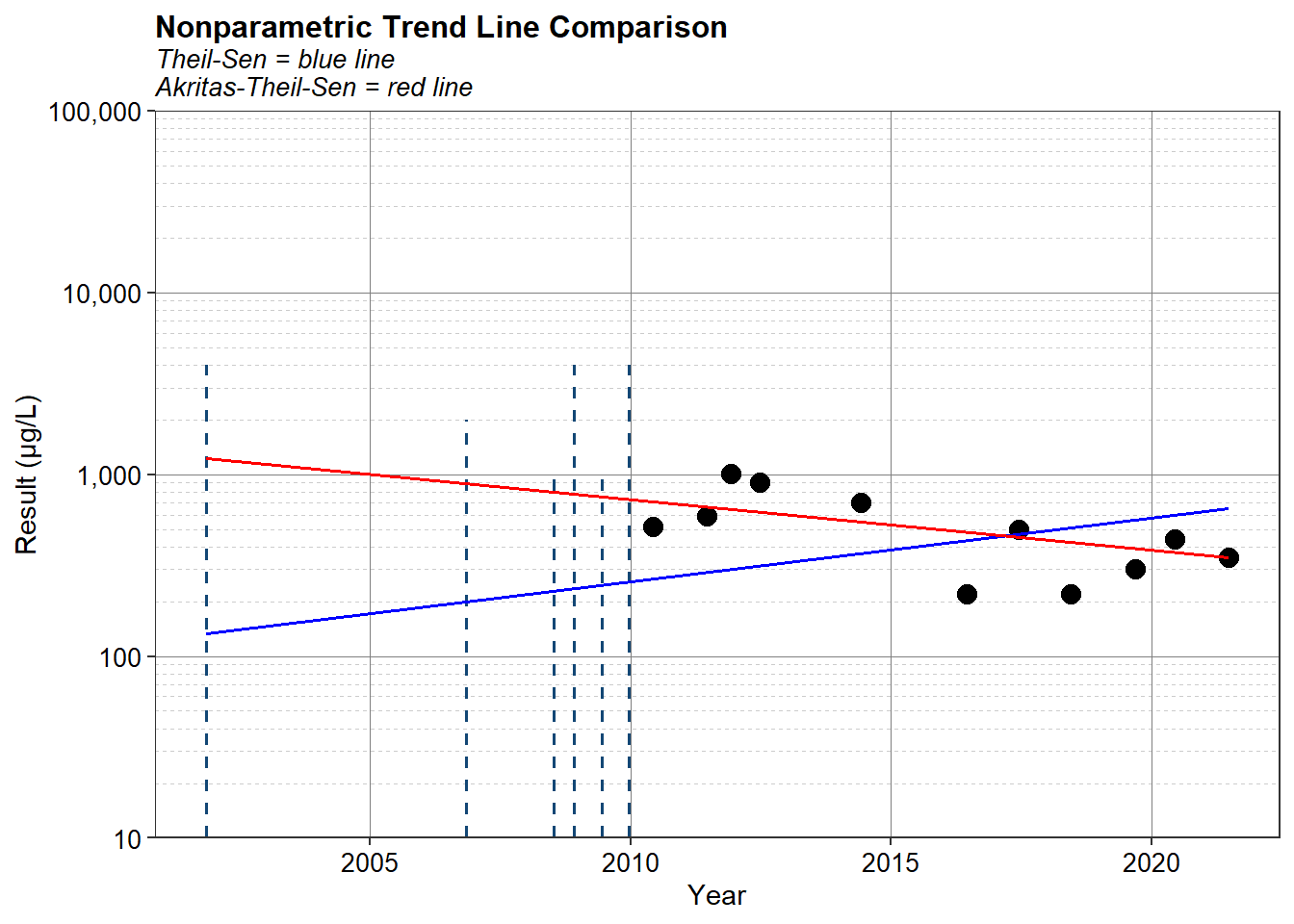
There are 17 total observations with 6 results that are non-detect, corresponding to a detection frequency of 64.7 percent. The p-value for the Mann-Kendall test is 0.035, which is less than the significance level of 0.05, indicating a statistically significant trend in concentrations. The Mann-Kendall test statistic S is 44, suggesting an increasing trend. The Theil-Sen estimate of slope is 16.1 µg/L/year, which also suggests an increasing trend in chloroform concentrations over time. The p-value for the ATS regression is 0.2, indicating no statistically significant correlation between time and concentration - the null hypothesis of no trend cannot be rejected. A time-series plot of the data and the two trend lines is shown below.

In the time-series plot, detected concentrations are shown as black circles and non-detects are shown as dashed vertical lines extending from zero to the censoring limit, which in this case, is the RL. Because non-detects are known to be within an interval between zero and the censoring limit, representing these values by an interval, provides a visual depiction of what is actually known about the data. The Theil-Sen and ATS trend lines are shown as solid blue and red lines, respectively. The plot is shown using a log base 10 scale for concentrations. Kendall’s tau and its test for significance are identical whether or not the test is conducted using log-transformed data or the original raw data. Log-transformed concentrations were used because the transformed data were judged to be more linear than on the original scale.

If used on data without non-detects, the slopes of the two methods should be very close if not exactly the same. However, the intercepts are computed in different ways. The EPA (2009) fits the line through the point (median of x, median of y) and then solves for the intercept. An alternative approach is to set the intercept as the median residual of all y values minus the slope*x (referred to as the Turnbull estimate of slope). This is a preferred approach because the Theil-Sen method of using the median of x and y individually is not necessarily a good center point of the entire data set. However, the Theil-Sen approach using the median slope to establish a line through a point located at the median concentration and median time of the data set was chosen in the 1980s likely because it was easier to compute.

Non-Detects Assigned One-Half the RL

The most common procedure for managing non-detects is substitution of some fraction of the detection or reporting limit. Although substitution is an easy method, it has no theoretical basis and it may impose new patterns of variation on the data, making statistical estimates inconsistent and yielding potentially misleading results. Contrary to the general rule of thumb, substitution of one-half the detection or reporting limit does not perform well even for low censoring levels. With that said, the trend analyses will be replicated but instead of assigning non-detects a common value less than the smallest detected result, the non-detects will be assigned one-half the RL. The results of the revised trend analyses are as follows:

# Subset data
dat <- dat %>%
  mutate(
    RESULT2 = ifelse(DETECTED == 'Y', RESULT, 0.5*RESULT)
  )

# Compute Statistics
cdat <- dat %>%
  summarize(
    Obs       = length(DATE),
    Dets      = sum(DETECTED == 'Y', na.rm = T),
    DetFreq   = round(Dets*100/Obs, 2),
    MK.S      = tryCatch(MannKendall(RESULT2)$S, error = function(e) NA),
    MK.P      = tryCatch(0.5*MannKendall(RESULT2)$sl, error = function(e) NA),
    TS.Slope  = tryCatch(theilsen(DATE, RESULT2)[2], error = function(e) NA),
    TS.Coeff  = tryCatch(theilsen(DATE, RESULT2)[1], error = function(e) NA),
    ATS.Tau   = tryCatch(cenken(RESULT, CENSORED, DATE)$tau, error = function(e) NA),
    ATS.P     = tryCatch(0.5*cenken(RESULT, CENSORED, DATE)$p, error = function(e) NA),
    ATS.Slope = tryCatch(cenken(RESULT, CENSORED, DATE)$slope, error = function(e) NA),
    ATS.Coeff = tryCatch(cenken(RESULT, CENSORED, DATE)$intercept, error = function(e) NA)
  )
print(data.frame(statistic = t(cdat)), digits = 2)

##            statistic
## Obs           17.000
## Dets          11.000
## DetFreq       64.710
## MK.S         -65.000
## MK.P           0.004
## TS.Slope     -51.123
## TS.Coeff  103374.344
## ATS.Tau       -0.147
## ATS.P          0.200
## ATS.Slope    -34.918
## ATS.Coeff  70936.594

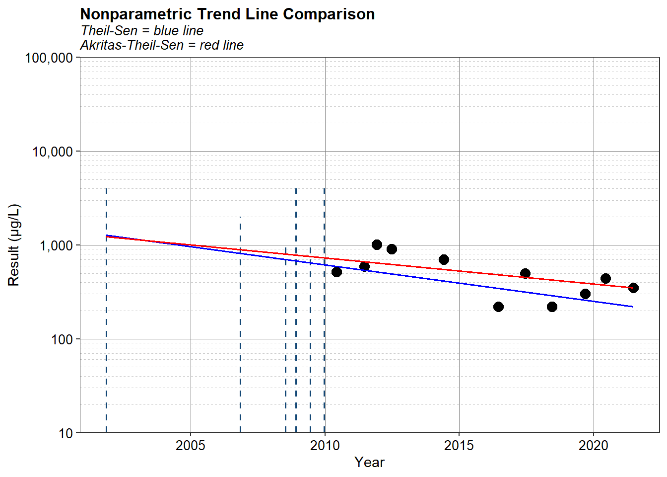
The p-value for the Mann-Kendall test is much lower at 0.004, and with a Mann-Kendall test statistic of -65, suggests a strongly decreasing trend in chloroform concentrations. This is supported by the Theil-Sen slope of -51.1 µg/L/year. This is compared to the p-value for the ATS regression of 0.2, indicating no statistically significant correlation between time and concentration. A time-series plot of the data and the two trend lines is shown below. Although the trend lines appear similar, the significance test for the ATS slope indicates no trend (p-value > 0.05) in chloroform concentrations over time. Remember that most of the earlier concentrations are censored observations (i.e., reported as non-detects). The only information known about these observations are that concentrations range within an interval between zero and the RL.

Conclusion

When non-detects are assigned an ad-hoc value, such as a common value less than the smallest detected value or some fraction of the RL, resulting statistics may be inaccurate and the amount and type of deviation is unknown. Ad-hoc substitution introduces structure to the data that is not in the actual population. Substitutions impose new patterns of variation on the data, making estimates of temporal trend inconsistent and yielding potentially misleading results. Fortunately, statistically robust procedures are available for analyzing censored data that make no assumptions or use of arbitrary values. For data with a high percentage of non-detects, ATS regression provides a better estimate of temporal trend because the Mann-Kendall test and Theil-Sen regression cannot be computed without substituting some unknown value for the non-detects.

References

Akritas, M.G., Murphy, S.A., Lavalley, M.P., 1995. The Theil-Sen estimator with doubly censored data and applications to astronomy. J. Am. Stat. Assoc. 90, 170-177.

Gilbert, R.O. 1987. Statistical Methods for Environmental Pollution Monitoring. Wiley, New York.

Helsel, D. R. 2012. Statistics for Censored Environmental Data using Minitab and R, 2nd edition. New York: John Wiley & Sons.

Hollander, M. and D.A. Wolf. 1973. Nonparametric Statistical Methods. Wiley, New York.

Kaplan, E.L. and O. Meier. 1958. Nonparametric Estimation from Incomplete Observations. J. Am. Stat. Assoc. 53, 457-481.

Kendall, M.G. 1975. Rank Correlation Techniques, 4th edition. Charles Griffen. London.

Mann, H.B. 1945. Nonparametric Tests Against Trend. Econometrica 13, 245-259.

Sen, P.K. 1968. Estimates of the regression coefficient based on Kendall’s tau. J. Am. Stat. Assoc. 63, 1379-1389.

Theil, H. 1950. A rank-invariant method of linear and polynomial regression analysis. Nederl. Akad. Wetensch, Proceed. 53, 386-392.

Turnbull, B.W., 1976. The empirical distribution function with arbitrarily grouped, censored andtruncated data. J. Royal Stat. Soc. Ser. B Methodol. 38, 290-295.

United States Environmental Protection Agency (EPA). 2009. Statistical Analysis of Groundwater Monitoring Data at RCRA Facilities: Unified Guidance. EPA-530-R-09-007. Office of Resource Conservation and Recovery, U.S. Environmental Protection Agency. March.