Introduction

An important objective of many environmental monitoring programs is to detect changes or trends in constituent concentrations over time. Many different statistical approaches are currently available for detecting and estimating trends that may be present in the data. These include simple correlation and regression analyses, time-series analyses, and methods based on nonparametric statistics. The Mann-Kendell (MK) test (Mann 1945; Kendall 1975; Gilbert 1987) is one of the most popular nonparametric tests for determining temporal trends. In general, nonparametric, or distribution-free, methods are recommended because they allow minimal assumptions to be made about the data. The MK test is well suited for analyzing non-normally distributed data and censored data, and data that have contain outliers or having missing observations. In this factsheet, the power of the MK test for trend detection is estimated by Monte Carlo simulation for various sample sizes and variability in the data.

Mann-Kendall Test

The purpose of the MK test is to statistically assess if there is a monotonic upward or downward trend of the variable of interest over time. A monotonic upward (downward) trend means that the variable consistently increases (decreases) through time, but the trend may or may not be linear. The test is based on the idea that a lack of trend should correspond to a time series plot fluctuating randomly about a constant mean level, with no visually apparent upward or downward pattern. The test compares the relative magnitudes of sample data rather than the data values themselves and thus, the underlying data do not need follow a specific distribution. Each data value is compared to all subsequent data values. Thus, the test can be viewed as a nonparametric test for zero slope of the linear regression of time-ordered data versus time, as illustrated by Hollander and Wolfe (1973, p. 201).

The MK test statistic (S) is found by counting the number of “concordant observations”, where the later-in-time observation has a larger value for the series, and subtracting the number of “discordant observations”, where the later-in-time observation has a smaller value for the series. This is done for all pairs of observations in the data set. The total difference is denoted S. Positive values of S indicate an increase in constituent concentrations over time, whereas negative values indicate a decrease in constituent concentrations over time. The strength of the trend is proportional to the magnitude of S (i.e., the larger the absolute value of S, the stronger the evidence for a real increasing or decreasing trend). Nondetects can be used in the test by assigning them a common value that is less than the smallest measured value in the data set (EPA 2009).

The calculated probability (p-value) for the MK test represents the probability that any observed trend would occur purely by chance (given the variability and sample size of the data set). Typically, a significance level of 0.05 (i.e., 95 percent confidence) is used to test the null hypothesis that there is no trend in the data. The significance level is the probability that a test erroneously detects a trend when none is present. The result of the MK test could be a significantly increasing or decreasing trend, or a nonsignificant result (the null hypothesis of no trend cannot be rejected).

Power Analysis

The significance level, or a Type I error, \(\alpha\), is the probability of rejecting the null hypothesis, when it is true. Significance levels are normally set quite low at values of 0.01, 0.05 or 0.10. The smaller the value of \(\alpha\), the more confidence there is that the null hypothesis is false when it has been identified as such. A Type II error ($\beta$) is the probability of accepting a null hypothesis, when it is false. The power of a test is the probability of correctly rejecting the null hypothesis, when it is false, which is equal to \(1 - \beta\).

Power is important to consider when conducting the MK test as it indicates the sensitivity of the test in detecting change. Because power is the probability of correctly rejecting the null hypothesis when it is false, it makes sense that we would like this as large as possible. Selecting a larger value of makes it easier to reject the null hypothesis of no trend and therefore increases the power of a test. Increasing the sample size increases the precision in the estimates and therefore increases the ability to detect differences in constituent concentrations and increases the power of the test.

Establishing an appropriate level of power when designing a monitoring program is as important as establishing the significance level of the test. If the power is too low, meaning the probability of rejecting the null hypothesis of no trend when in fact there is a trend, the performance of the test suffers. In many cases, a power from 0.8 to 0.9 (80 to 90 percent) is considered appropriate for detecting a temporal trend when using the MK test.

The power of a test can be determined only when the true situation is known. In a trend test, this requires knowledge of the trend. Let’s create a function in the R statistical language that generates a data set exhibiting either a linear trend with a constant rate of decrease, or a first-order decay. Then, let’s test the function assuming a starting concentration of 100 units with a constant rate of decrease of 4 units across 8 sampling events.

# Load libraries
library(tidyr)
library(dplyr)
library(purrr)
library(ggplot2)

# Function to generate trend
generate_trend <- function(n, mu1, k, type = 'lin') {
  i <- 1:n
  if (type == 'lin') {
    k <- k * (1 - n)
    b <- k / (n - 1)
    mu <- mu1 + (i - 1) * b
  }
  if (type == 'exp') {
    mu <- mu1 * exp(k * (i - 1))
  }
  data.frame(i, mu)
}

# Generate data with trend
dt_lin <- generate_trend(n = 8, mu1 = 100, k = 4, type = 'lin')
print(dt_lin)

##   i  mu
## 1 1 100
## 2 2  96
## 3 3  92
## 4 4  88
## 5 5  84
## 6 6  80
## 7 7  76
## 8 8  72

Now, let’s test the function assuming a first-order decay with a decay rate of -0.07 per unit time.

# Generate data with trend
dt_exp <- generate_trend(n = 8, mu1 = 100, k = -0.07, type = 'exp')
print(dt_exp)

##   i        mu
## 1 1 100.00000
## 2 2  93.23938
## 3 3  86.93582
## 4 4  81.05842
## 5 5  75.57837
## 6 6  70.46881
## 7 7  65.70468
## 8 8  61.26264

The probability of rejecting the null hypothesis of no trend when in fact there is a trend (the power of the test) can be computed by Monte Carlo simulation for a chosen level of \(\alpha\). Let’s create a function within the R statistical language for performing Monte Carlo simulation to observe the power of the MK test using 1000 independent time series for each sample size, where the time series exhibits a pre-specified trend. To replicate actual measurements, let’s add a normally distributed error (noise) to each observation in the time series assuming different values for the variance.

# Function to estimate power
power_trend <- function(n, mu, sd, alpha = 0.05, nsims = 100) {
  pval <- numeric(nsims)
  for(j in 1:nsims) {
    y <- rnorm(n = n, mean = mu, sd = sd)
    pval[j] = 0.5 * Kendall::MannKendall(y)$sl[[1]]
  }
  power <- sum(pval < alpha) / nsims

  return(power)
}

Let’s create a function to plot the simulation results.

get_plot <- function(dd, type, mu1, k) {

  # Create subtitle
  sub_title <- ifelse(
    type == 'lin',
    paste0('C = ', mu1, '; -', k, ' unit change per sampling event'),
    paste0('C = ', mu1, '; ', k, ' first-order decay rate')
  )

  # Plot the results
  p <- ggplot(data = dd, aes(x = n, y = power, color = as.factor(sd))) +
    geom_line(size = 1) +
    scale_x_continuous(limits = c(4, 20),
                       breaks = seq(4, 20, 4),
                       minor_breaks = seq(4, 20, 1)) +
    scale_y_continuous(limits = c(0, 1),
                       breaks = seq(0, 1, 0.2),
                       minor_breaks = seq(0, 1, .1)) +
    labs(title = paste0('Power of the Mann-Kendall test as a function of sample size ',
                        'for different\n', 'values of the standard deviation'),
         subtitle = sub_title,
         color = paste0('Standard\n', 'Deviation'),
         x = 'Sample Size',
         y = 'Power\n') +
    scale_color_hue(l = 50) +
    theme_bw() +
    theme(plot.title = element_text(margin = margin(b = 3), size = 12,
                         hjust = 0.0, color = 'black', face = quote(bold)),
          plot.subtitle = element_text(margin = margin(b = 3), size = 11,
                            hjust = 0.0, color = 'black', face = quote(italic)),
          axis.title.y = element_text(size = 12, color = 'black'),
          axis.title.x = element_text(size = 12, color = 'black'),
          axis.text.x = element_text(size = 11, color = 'black'),
          axis.text.y = element_text(size = 11, color = 'black'),
          legend.position = c(0.90, 0.13),
          legend.title = element_text(size = 11, face = quote(bold)),
          legend.text = element_text(size = 10))

  return(p)
}

For our first simulation, let’s assume a linear trend with a constant rate of decrease of 4 units, an initial concentration of 100 units, and an \(\alpha\) equal to 0.05. Well will calculate the power of the MK test as a function of sample size for different values of the sample standard deviation.

# Combine generate trend and power of trend functions into single function
get_power <- function(n, mu1, sd, k, type, alpha, nsims) {
  dat <- generate_trend(n = n, mu1 = mu1, k = k, type = type)
  pout <- power_trend(n = n, mu = dat$mu, sd = sd, alpha = alpha, nsims = nsims)

  return(pout)
}

# Create input file for nobs and sd
sd <- c(4, 6, 10)
nobs <- seq(4, 20, by = 1)
input <- expand.grid(nobs, sd)
names(input) <- c('n', 'sd')

# Get power as function of sd and nobs using map2 function
type <- 'lin'
mu1 <- 100
k <- 4
pout <- 
  input %>%
  mutate(
    power = map2(
      n, sd, get_power, mu1 = mu1, k = k, type = type,
      alpha = 0.05, nsims = 1000
    )
  ) %>%
  unnest()

Let’s plot the results of the simulation.

get_plot(dd = pout, type = type, mu1 = mu1, k = k)

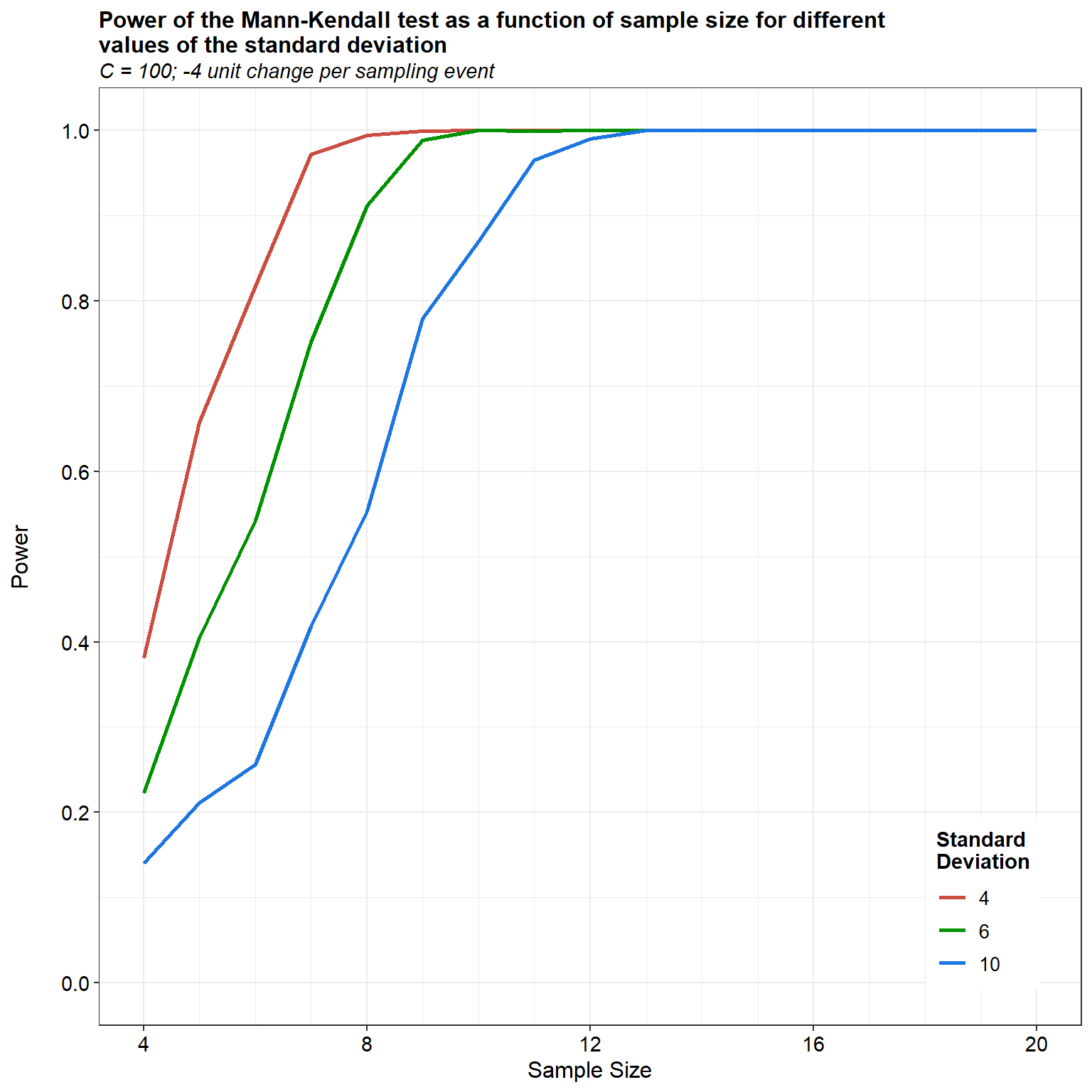
The results of the simulation indicate that the power of the MK test depends on the sample size and the amount of variation within the time series. As the sample size increases, the test becomes more powerful; however, the power of the test decreases as the amount of variation increases within the time series.

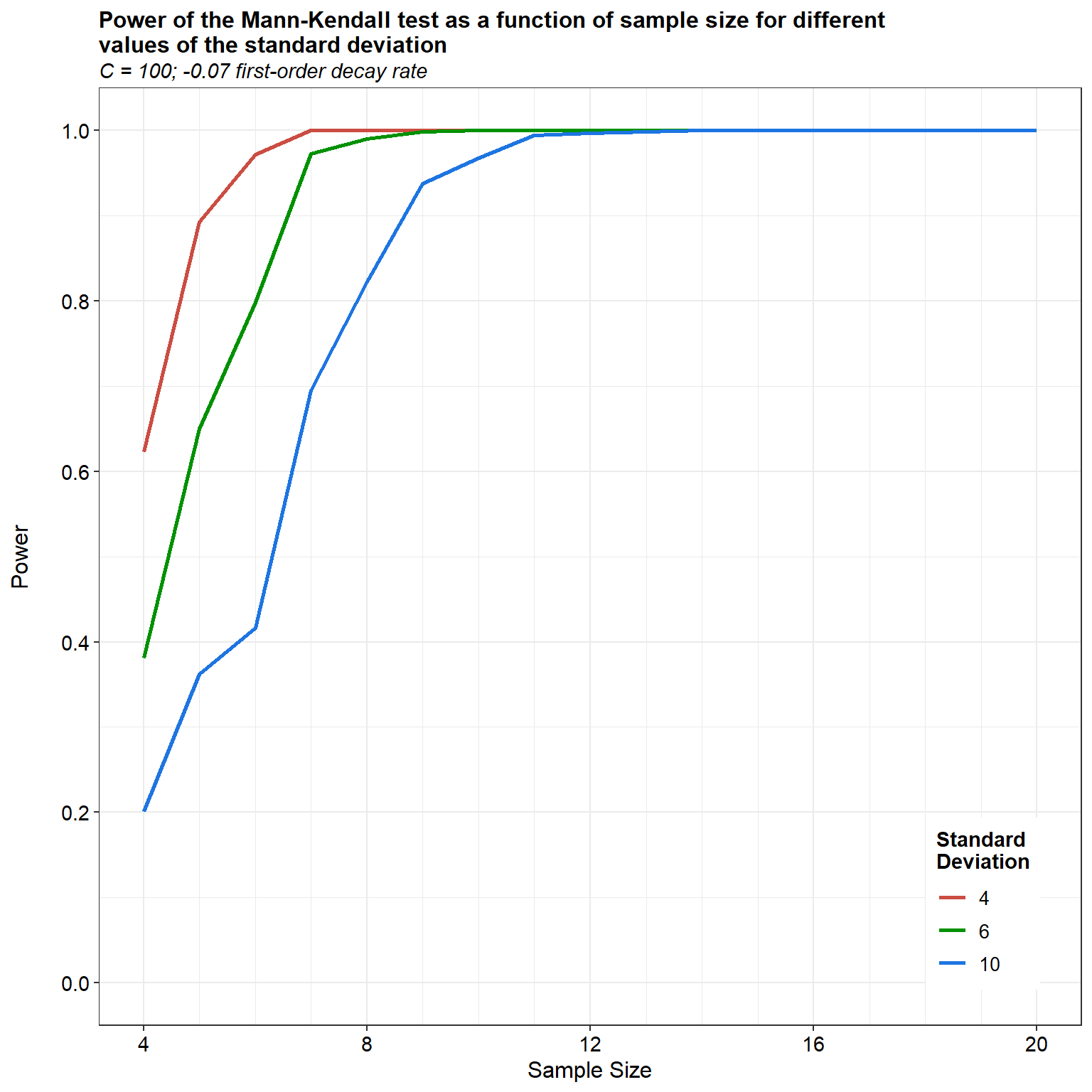
For our second simulation, let’s assume an exponential trend with a first-order rate constant of -0.07 per unit time, an initial concentration of 100 units, and an \(\alpha\) equal to 0.05.

# Get power as function of sd and nobs using map2 function
type <- 'exp'
mu1 <- 100
k <- -0.07
pout <- 
  input %>%
  mutate(
    power = map2(
      n, sd, get_power, mu1 = mu1, k = k, type = type,
      alpha = 0.05, nsims = 1000
    )
  ) %>%
  unnest()

# Create subtitle
sub_title <- ifelse(
  type == 'lin',
  paste0('C = ', mu1, '; -', k, ' unit change per sampling event'),
  paste0('C = ', mu1, '; ', k, ' first-order decay rate')
)

# Plot the results
get_plot(dd = pout, type = type, mu1 = mu1, k = k)

For our last simulation, let’s assume an exponential trend with a first-order rate constant of -0.1 per unit time, an initial concentration of 100 units, and an \(\alpha\) equal to 0.05.

# Get power as function of sd and nobs using map2 function
type <- 'exp'
mu1 <- 100
k <- -0.1
pout <- 
  input %>%
  mutate(
    power = map2(
      n, sd, get_power, mu1 = mu1, k = k, type = type,
      alpha = 0.05, nsims = 1000
    )
  ) %>%
  unnest()

# Plot the results
get_plot(dd = pout, type = type, mu1 = mu1, k = k)

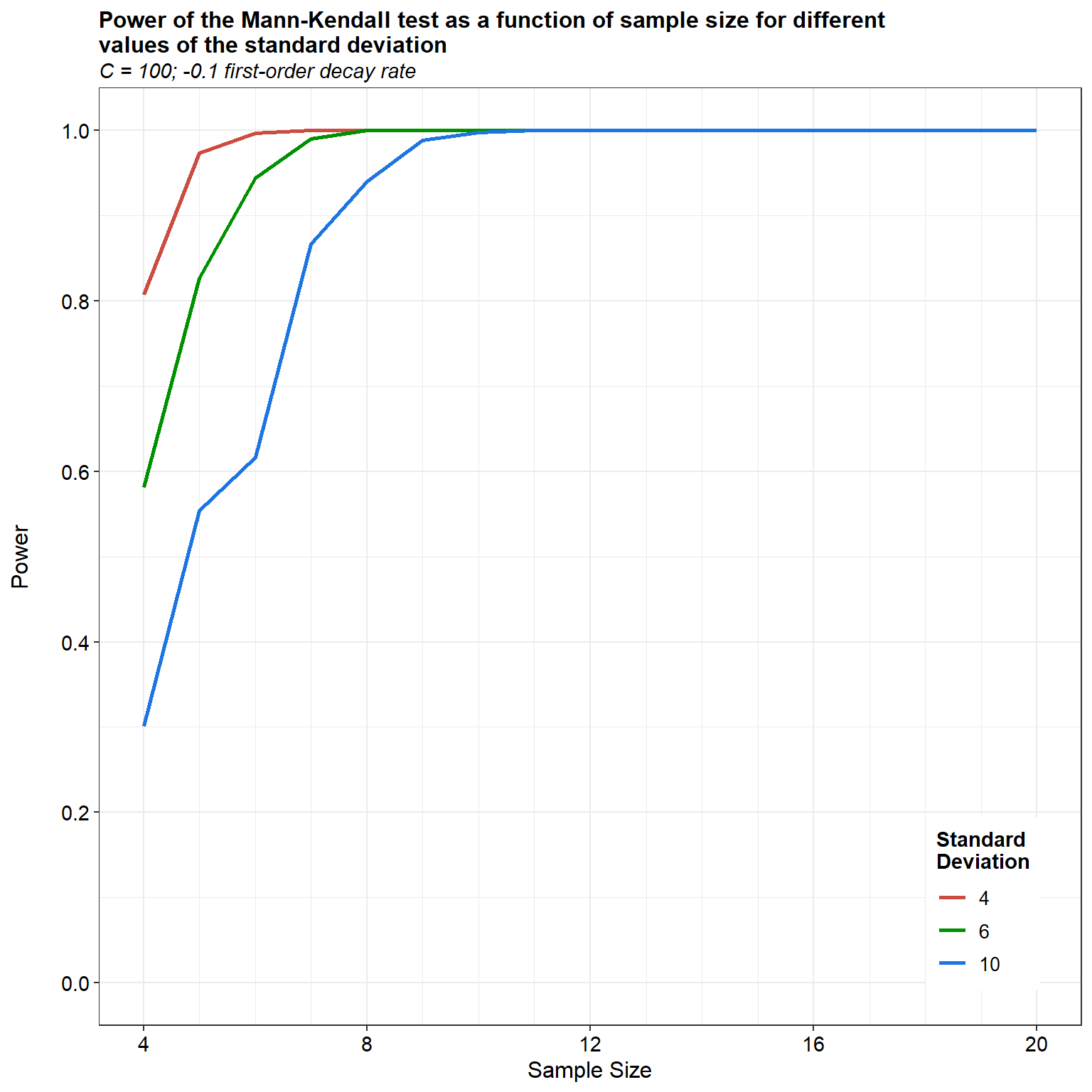
Simulation results assuming similar initial conditions but using a first-order rate constants of -0.07 and -0.1 per unit time indicate that the power of the MK test also depends on the magnitude of the trend; the larger the absolute magnitude of the trend, the more powerful the test.

Conclusions

Statistical power of the MK test can be increased by increasing sample size or by reducing the variation (noise) in the data. When the variation in the data is low, the power of the MK test increases sharply with sample size; however, the test cannot effectively detect small temporal differences in time series containing large variation in the data. Power also can be increased by reducing the significance level of the test, although this will increase the false positive rate of the test. Typically, the power of the MK test will be low for sample sizes below about 8.

A few considerations worth noting is that we assume there are no nondetects in the data and that the data are independent. If nondetects are expected in the resulting data, then the value of the computed power is only an approximation to the correct value. This approximation will tend to be less accurate as the number of nondetects increases. The MK test assumes minimal autocorrelations in the data. Many environmental processes show some degree of autocorrelation, and if present, there is a chance that the MK test would suggest a trend, when in fact the trend significance is due to autocorrelation. A method to control for autocorrelation is to fit an autoregressive model to the time series, then perform the trend test on the residuals using proper transformations.

Yue et al. (2002) found that the power of the MK test is dependent upon distribution type. The lowest power was reported to be associated with a lognormal distribution. This is an interesting result indicating that the power of the MK test is dependent on the distribution type, in contrast to common thinking that states that this test is distribution free. Because most environmental data are thought to be lognormally distributed, such increases/decreases in power may inadvertently affect the interpretation of significance, especially when comparing variables that have different statistical properties.

Final Thoughts

Daniel (1978) has discussed the difference between statistical significance and practical significance. He noted that a statistically significant trend may not be practically significant and vice versa. Sufficiently large samples will reveal any change, no matter how small, using a statistical test, but this may not be of any practical significance. Likewise, small samples may fail to detect a change statistically, but the degree of change might be of practical significance.

References

Daniel, W.W. 1978. Applied Nonparametric Statistics. Houghton Mifflin, Boston.

Gilbert, R.O. 1987. Statistical Methods for Environmental Pollution Monitoring. Wiley, New York.

Hollander, M. and D.A. Wolf. 1973. Nonparametric Statistical Methods. Wiley, New York.

Kendall, M.G. 1975. Rank Correlation Methods, 4th Edition. Charles Griffin, London.

Mann, H.B. 1945. Non-parametric tests against trend. Econometrica 13, 163-171.

United States Environmental Protection Agency (EPA). 2009. Statistical Analysis of Groundwater Monitoring Data at RCRA Facilities: Unified Guidance. EPA-530-R-09-007. Office of Resource Conservation and Recovery, U.S. Environmental Protection Agency. March.

Yue, S., P. Pilon, and G. Caradias. 2002. Power of the Mann-Kendall and Spearman’s rho tests for detecting monotonic trends in hydrological series. J. Hydrol. 259, 254-271.