Plume Moment Analysis Using Thiessen Polygons
By Charles Holbert
April 2, 2022
Introduction
The behavior of contaminants in groundwater can be assessed by evaluating how mass and the spatial extent of mass change through time. This post describes methods that can be used to evaluate contaminant concentrations measured in wells to determine plume mass and plume center-of-mass. The evaluation provides spatial and temporal information about plume behavior. At most groundwater remediation sites, the contaminant plume is not controlled exclusively by natural processes but is also affected by remedial activities implemented at the site. A decrease in plume mass can indicate that (1) the source strength has been reduced by some remedial effort; (2) the plume is naturally attenuating; or most likely (3) both the source strength has been reduced and the plume is naturally attenuating. A decrease in plume mass over time and a stable center-of-mass suggest that the assimilative capacity of the aquifer exceeds mass flow out of the source area and the plume is attenuating.
Mass-based analyses of groundwater contaminants provide complementary information not readily quantified using single-well analytics. For example, when evaluating different areas within a dissolved-phase plume, statistical trends in contaminant concentrations may produce conflicting results that make it difficult to assess the overall condition of the plume. An assessment of total integrated mass and center-of-mass over time provides a quantitative measure of the overall plume. Spatial moment analysis as described here can be used for a variety of purposes, including an evaluation of natural attenuation processes, as a measure of performance for existing remedies, to estimate remedial timeframes, and for remedial system optimization.
The Thiessen polygon method for conducting spatial moment analysis assumes that the contaminant plume can be represented by multiple polygons of defined area \((A_n)\), thickness \((h_n)\), and concentration \((C_n)\). Thiessen polygons are applied as a standard technique in geography and hydrology to assign a zone of influence or representativeness to an area around a point. Thus, each of the Thiessen polygonal areas can be considered as the area-of-influence for the corresponding monitoring well. For ease of calculation, the analysis is conducted in two dimensions (2-D) and aquifer thickness is assumed constant across the region of investigation.
Background
Spatial moment analysis was introduced by Aris (1956) to study the dispersion of a solute in a fluid flowing through a tube. Later, Marle et al. (1967) and Guven et al. (1984) used this method to analyze transport of non-reactive solutes for steady horizontal flow in a perfectly stratified aquifer. Freyberg (1986) proposed using spatial moments to develop estimates of total mass and center-of-mass in a groundwater contaminant plume. Dupont (1998) used spatial moment analysis to assess intrinsic remediation and plume stability for a petroleum contaminated groundwater plume at Hill Air Force Base, in Utah. The Monitoring and Remediation Optimization System (MAROS) software (AFCEE 2002), developed in 1998 for the United States Air Force as a decision support system for optimizing groundwater monitoring, contains a formalized spatial moment analysis procedure to assess plume stability. Hyman and Dupont (2001) proposed using spatial moment analysis as a natural attenuation assessment method. Gorder et al. (2006) used spatial moments to evaluate remedial system performance and remedial process optimization at a site contaminated with dense nonaqueous phase liquids. Brauner et al. 2008 demonstrated the use of spatial moments for evaluating dissolved plume stability, remediation timeframes, and long-term sustainability of natural attenuation processes at dissolved chlorinated solvent contamination sites. Gorder and Holbert (2010) presented a computer software tool for evaluating plume dynamics using spatial moment analysis.
Spatial moment analysis provides a relative measure of plume dynamics. Statistical trend analysis of the spatial moments provides an overall assessment of plume stability for each groundwater contaminant. This information is useful in understanding how the plume may evolve in the future. The approach outlined below was developed to assess stability of groundwater plumes based on scientifically sound, quantitative analyses of current and historical site groundwater conditions.
Plume Mass and Plume Center-of-Mass
Plume mass, plume center-of-mass, and the spread of the contaminant about the center-of-mass can be viewed as the zeroth, first, and second spatial moment of concentration, respectively. The ijkth moment of the contaminant concentration distribution in space \(M_{ijk} (t)\) is defined as (Freyburg 1986):
\begin{equation}
 M_{ijk}(t) = \int_{-\infty}^{\infty} \int_{-\infty}^{\infty} \int_{-\infty}^{\infty} \eta C(x,y,z,t) x^i y^j z^k\ dxdydz
 \end{equation}
where \(\eta\) denotes porosity, assumed to be a constant for ease of computation; and x, y, z are the spatial coordinates, respectively, corresponding to easting, northing, and elevation; i, j, and k determine the order of the moment; and C(x,y,z) is a continuous function of space describing the distribution of contaminant concentration.
Because the concentration data are spatially discontinuous, the function C(x,y,z) is unknown and must be estimated using measurements at discrete locations (i.e., from measured concentrations in samples taken from n = 1, 2,…, N wells at locations \((x_n, y_n, z_n)\)). Using the discrete measurements, the spatial moments can be approximated by the following expression:
\begin{equation}
 \hat{M}_{i,j,k} = \sum_{n = 1}^{Nwells} \eta C_n x^i y^j z^k A_n
 \end{equation}
where \(C_n\) is the contaminant concentration in the \(n^{th}\) well and \(A_n\) is an area associated with the \(n^{th}\) well. The plume mass is given by the zeroth moment and can be estimated with the following:
\begin{equation}
 Mass \approx \hat{M}_{0,0,0} = \sum_{n = 1}^{Nwells} \eta C_n h_n A_n
 \end{equation}
where \(h_n\) is the estimated vertical thickness of the plume at each area \(A_n\).
The zeroth moment is the sum of individual mass estimates derived from concentrations for all monitoring wells and is an estimate of the total dissolved mass in the plume. The zeroth moment calculation can show high variability over time, largely due to the fluctuating concentrations at the most contaminated wells as well as the varying number and identity of wells in the network. Plume analysis and delineation based exclusively on concentration can exhibit temporal and spatial variability. The mass estimate is also sensitive to the extent of the site monitoring well network over time. Therefore, the plume should be adequately delineated for mass estimates to be considered.
The 2-D coordinates \((X_c, Y_c)\) of the center-of-mass (also denoted as the centroid) for each sample event and contaminant are based on the first spatial moments:
\begin{equation}
 X_c = \frac{\hat{M}_{1,0}}{\hat{M}_{0,0}} = \frac{\int \int \eta C_i x\; dxdy}{\int \int \eta C_i \; dxdy}
 \end{equation}
and
\begin{equation}
 Y_c = \frac{\hat{M}_{0,1}}{\hat{M}_{0,0}} = \frac{\int \int \eta C_i y\; dxdy}{\int \int \eta C_i \; dxdy}
 \end{equation}
Similar to the zeroth moment calculation, the data are spatially discontinuous and require a numerical approximation as follows:
\begin{equation}
 X_c \approx \frac{\hat{M}_{1,0}}{\hat{M}_{0,0}} = \frac{\sum x_n C_n A_n}{\sum C_n A_n}
 \end{equation}
and
\begin{equation}
 Y_c \approx \frac{\hat{M}_{0,1}}{\hat{M}_{0,0}} = \frac{\sum y_n C_n A_n}{\sum C_n A_n}
 \end{equation}
The longitudinal and transverse dispersive spreading of the dissolved-phase plume can be evaluated from the second-order moments. The second-order moments are not discussed here because these numbers can not be readily compared with a physical measurement of dissolved plumes.
The changing center-of-mass locations indicate the movement of the center-of-mass over time. Analysis of the movement of mass should be viewed as it relates to (1) the original source location of contamination, (2) the direction of groundwater flow, and (3) the location of any remedial activities conducted at the site. Spatial and temporal trends in the center-of-mass can indicate spreading or shrinking or transient movement based on seasonal variation. If the center-of-mass is located at increasing downgradient distances for consecutive monitoring events, this indicates plume expansion. If the center-of-mass is located at decreasing downgradient distances for consecutive monitoring events, this indicates plume shrinkage. No appreciable movement in center-of-mass would indicate plume stability.
Interpretation of the spatial moments must account for both the zeroth and first moments. For example, a first moment trend away from the original source location might suggest the plume is expanding. If during the same time the zeroth moment indicates an overall decreasing plume mass, the data would be consistent with a plume whose core is being attenuated more rapidly than the distal portion of the plume.
To calculate the distance from the center-of-mass of the plume for a particular contaminant and monitoring event to the source location, \(D_{src}\), the following formula can be used:
\begin{equation}
 D_{src} = \sqrt{(X_{src} - X_c)^2 + (Y_{src} - Y_c)^2}
 \end{equation}
where \(X_c\) and \(Y_c\) are the coordinates of the center-of-mass; and \(X_{src}\) and \(Y_{src}\) are the coordinates of the source location for the particular contaminant under consideration. If the source is not well define, or the site contains multiple source locations, the change in center-of-mass can be compared to the initial estimated center-of-mass location. In this case, the distance from the center-of-mass of the plume for a particular contaminant and monitoring event to the initial location is given by:
\begin{equation}
 D_{src} = \sqrt{(X_{co} - X_c)^2 + (Y_{co} - Y_c)^2}
 \end{equation}
where \(X_{co}\) and \(Y_{co}\) are the coordinates of the initial center-of-mass location for the particular contaminant under consideration. The bearing angle also can be calculated from the initial center-of-mass location \((X_{co}, Y_{co})\) to a subsequent center-of-mass location \((X_{c}, Y_{c})\). This bearing angle is measured in the clockwise direction from due north. This provides both a distance and direction by which the dissolved-phase center-of-mass has changed over time, relative to the initial center-of-mass location.
Moment analysis can be used to evaluate multiple groundwater contaminants to provide a quick way of comparing the size and movement of contaminant masses relative to one another. An overall plume condition can be determined for each contaminant based on a statistical trend analysis of the moments for each monitoring event. For example, the moment trends over time can be assessed by the Mann-Kendall test (Mann 1945; Kendall 1975; Gilbert 1987). The Mann-Kendall test is based on the idea that a lack of trend should correspond to a time series plot fluctuating randomly about a constant mean level, with no visually apparent upward or downward pattern (USEPA 2009). As a nonparametric procedure, the test does not require any assumptions as to the statistical distribution of the data (e.g., normal, lognormal, etc.) and can be used with data that include irregular sampling intervals and missing values.
A word of caution is in order with respect to spatial moment analysis. If the same wells are sampled during each monitoring event, the calculated spatial moments will be accurate reflections of the dissolved-phase contaminant plume over time (within achieved error limits for field sampling and laboratory analysis). However, if different wells are sampled over time, then variation in the calculated moments may be a result of actual variations in the moments over time, variation in the wells sampled over time, or both.
Thiessen Polygon Area
The areas \(A_n\) used in the moment analysis depend on the method used to subdivide the plume into discrete regions associated with wells. The method applied here is based on Thiessen polygons (also referred to as Dirichlet tessellation, or Voronoi diagrams) obtained by Delaunay triangulation (Ripley 2004) of the monitoring well network. Thiessen polygon analysis is a technique for quantifying a spatially distributed feature represented by unevenly distributed observation points (Brassel and Reif 1979). Thiessen polygons have many applications in statistics and data analysis. Statistical applications range from its use as a computational technique in distance-based methods of point pattern analysis, through the use of tessellation statistics such as contiguity lengths, to the investigation of tessellation-based models for the spread of infectious disease (Sibson 1980).
The basis of the Thiessen polygon method as used for plume moment analysis was developed in the field of hydrology for estimating areas associated with point rainfall measurements within rain gage networks (Chow et al. 1988). The method assumes the concentration measured at a given sampling point is constant out to a distance halfway to the sampling points located next to it in all directions. The relative weights (areas) represented by each sampling point are determined by the construction of a Thiessen polygon network, the boundaries of which are formed by the perpendicular bisectors of lines connecting adjacent points (Hymand and Dupont 2001). The outer boundary of the Thiessen polygon network is estimated based on the outermost well locations.
A simple example of both Delaunay triangulation (solid red lines) and Thiessen polygons (dashed black lines) for 10 points is shown in Figure 1. Note that each dashed black line is the perpendicular bisector of a red line. The area within each cell is closer to the point within the cell than any other point in the plot. For a given set of points, the Thiessen polygons are always unique.
# Load libraries
library(deldir)

# Set seed for reproducibility
set.seed(10)

# Create some data
x <- sample(1:200, 10)
y <- sample(1:200, 10)
pts <- data.frame(
  id = 1:10,
  x, y
)

# Create plot of the triangulation and tessellation
dxy <- deldir(x, y)
par(mar = c(0, 0, 0, 0))
plot(
  dxy,
  wl = 'both',
  cmpnt_col = c('red', 'black'),
  cmpnt_lty = c(1, 2)
)
points(x, y, pch = 16, cex = 1.2, col = 'black')
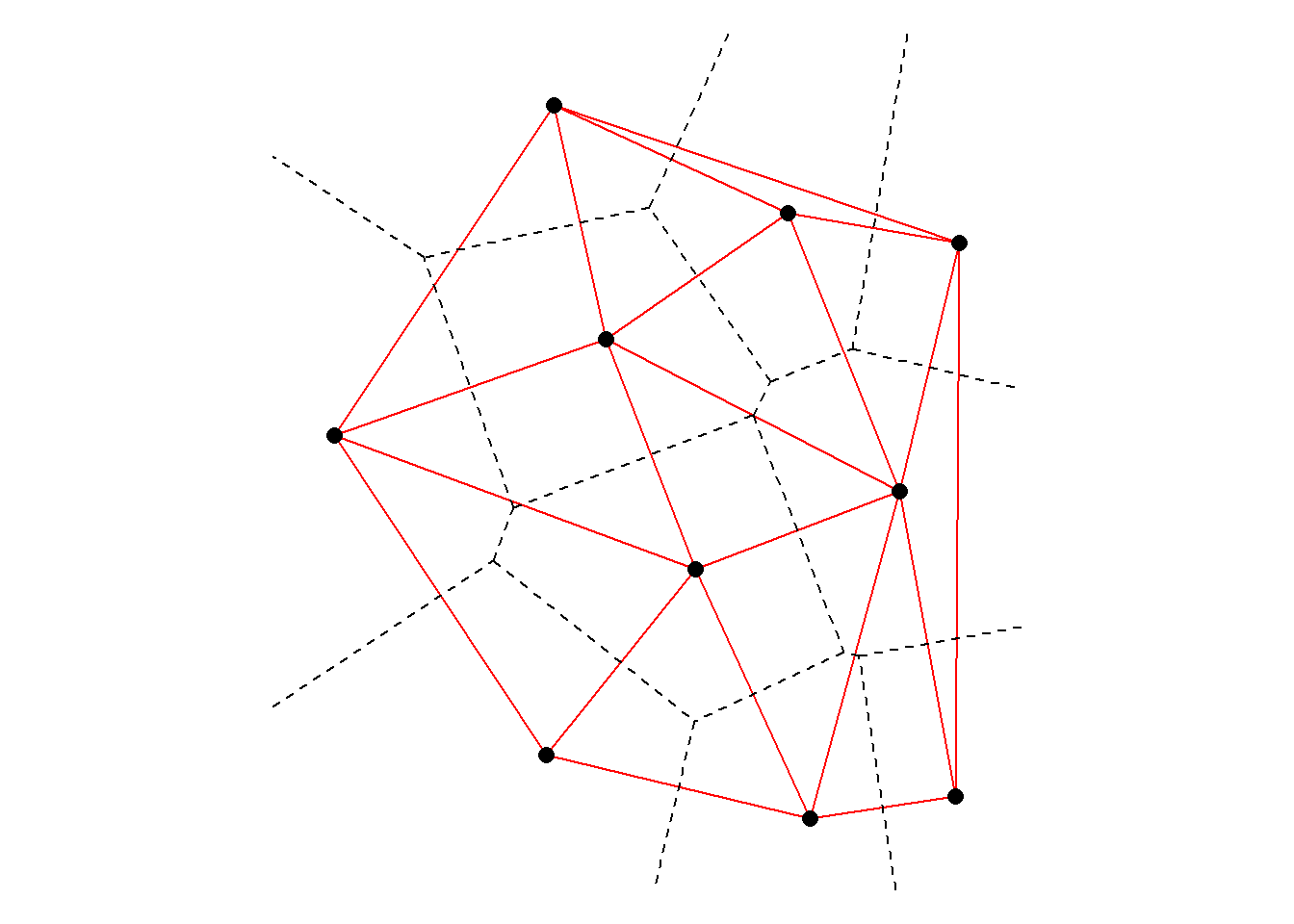
Figure 1: Delaunay triangulation (solid red lines) and Thiessen polygons (dashed black lines).
# Load libraries
library(PBSmapping)
library(sp)

# Create clipped polygons
XY <- cbind.data.frame(
  PID = 1,
  POS = 1:length(pts$x),
  X = pts$x,
  Y = pts$y,
  ID = pts$id
)

# Extend range by 150 percent for polygons before clipping
polys <- calcVoronoi(
  XY,
  xlim = extendrange(pts$x, f = 1.5),
  ylim = extendrange(pts$y, f = 1.5)
)

# Find the convex hull points and calculate centroid
hull <- calcConvexHull(XY, keepExtra = FALSE)
cent <- calcCentroid(hull, rollup = 3)

# Calculate the boundary points using the supplied buffer value
buff = 0.10

for (i in 1:length(hull$X)) {
  opp = hull$Y[i] - cent$Y
  adj = hull$X[i] - cent$X
  if (hull$X[i] >= cent$X && hull$Y[i] >= cent$Y) quad = 1
  if (hull$X[i] >= cent$X && hull$Y[i] < cent$Y) quad = 2
  if (hull$X[i] < cent$X && hull$Y[i] < cent$Y) quad = 3
  if (hull$X[i] < cent$X && hull$Y[i] >= cent$Y) quad = 4
  alpha = abs(atan2(opp,adj))
  if (quad == 3 || quad == 4) alpha = pi-alpha
  dist = ((hull$Y[i] - cent$Y)^2 + (hull$X[i] - cent$X)^2)^0.5
  addhyp = dist * buff
  addx = abs(addhyp * cos(alpha))
  addy = abs(addhyp * sin(alpha))
  if (quad == 1) {
      hull$X[i] = hull$X[i] + addx
      hull$Y[i] = hull$Y[i] + addy
  }
  if (quad == 2) {
      hull$X[i] = hull$X[i] + addx
      hull$Y[i] = hull$Y[i] - addy
  }
  if (quad == 4) {
      hull$X[i] = hull$X[i] - addx
      hull$Y[i] = hull$Y[i] + addy
  }
  if (quad == 3) {
      hull$X[i] = hull$X[i] - addx
      hull$Y[i] = hull$Y[i] - addy
  }
}
polysclip <- joinPolys(hull, polys, "INT")

# Generate SpatialPolygons file in order to create shapefile
lst <- list()
np <- which(polysclip$POS == 1)
for (i in 1:length(np)) {
  if (i < length(np)) {
    r <- Polygons(list(Polygon(cbind(c(polysclip[np[[i]]:(np[[i+1]]-1),3],
                                       polysclip[np[[i]],3]),
                                     c(polysclip[np[[i]]:(np[[i+1]]-1),4],
                                       polysclip[np[[i]],4])
                                     )
                               )
                       ), ID = pts[i, 1])
  }
  else {
    r <- Polygons(list(Polygon(cbind(c(polysclip[np[[i]]:length(polysclip$X),3],
                                       polysclip[np[[i]],3]),
                                     c(polysclip[np[[i]]:length(polysclip$X),4],
                                       polysclip[np[[i]],4])
                                    )
                              )
                      ), ID = pts[i, 1])
  }
    lst <- c(lst, list(r))
}
sr1 <- SpatialPolygons(lst)
# Load libraries
library(PBSmapping)
library(sp)

# Create clipped polygons
XY <- cbind.data.frame(
  PID = 1,
  POS = 1:length(pts$x),
  X = pts$x,
  Y = pts$y,
  ID = pts$id
)

# Extend range by 150 percent for polygons before clipping
polys <- calcVoronoi(
  XY,
  xlim = extendrange(pts$x, f = 1.5),
  ylim = extendrange(pts$y, f = 1.5)
)

# Find the convex hull points and calculate centroid
hull <- calcConvexHull(XY, keepExtra = FALSE)
cent <- calcCentroid(hull, rollup = 3)

# Calculate the boundary points using the supplied buffer value
buff = 1

for (i in 1:length(hull$X)) {
  opp = hull$Y[i] - cent$Y
  adj = hull$X[i] - cent$X
  if (hull$X[i] >= cent$X && hull$Y[i] >= cent$Y) quad = 1
  if (hull$X[i] >= cent$X && hull$Y[i] < cent$Y) quad = 2
  if (hull$X[i] < cent$X && hull$Y[i] < cent$Y) quad = 3
  if (hull$X[i] < cent$X && hull$Y[i] >= cent$Y) quad = 4
  alpha = abs(atan2(opp,adj))
  if (quad == 3 || quad == 4) alpha = pi-alpha
  dist = ((hull$Y[i] - cent$Y)^2 + (hull$X[i] - cent$X)^2)^0.5
  addhyp = dist * buff
  addx = abs(addhyp * cos(alpha))
  addy = abs(addhyp * sin(alpha))
  if (quad == 1) {
      hull$X[i] = hull$X[i] + addx
      hull$Y[i] = hull$Y[i] + addy
  }
  if (quad == 2) {
      hull$X[i] = hull$X[i] + addx
      hull$Y[i] = hull$Y[i] - addy
  }
  if (quad == 4) {
      hull$X[i] = hull$X[i] - addx
      hull$Y[i] = hull$Y[i] + addy
  }
  if (quad == 3) {
      hull$X[i] = hull$X[i] - addx
      hull$Y[i] = hull$Y[i] - addy
  }
}
polysclip <- joinPolys(hull, polys, "INT")

# Generate SpatialPolygons file in order to create shapefile
lst <- list()
np <- which(polysclip$POS == 1)
for (i in 1:length(np)) {
  if (i < length(np)) {
    r <- Polygons(list(Polygon(cbind(c(polysclip[np[[i]]:(np[[i+1]]-1),3],
                                       polysclip[np[[i]],3]),
                                     c(polysclip[np[[i]]:(np[[i+1]]-1),4],
                                       polysclip[np[[i]],4])
                                     )
                               )
                       ), ID = pts[i, 1])
  }
  else {
    r <- Polygons(list(Polygon(cbind(c(polysclip[np[[i]]:length(polysclip$X),3],
                                       polysclip[np[[i]],3]),
                                     c(polysclip[np[[i]]:length(polysclip$X),4],
                                       polysclip[np[[i]],4])
                                    )
                              )
                      ), ID = pts[i, 1])
  }
    lst <- c(lst, list(r))
}
sr2 <- SpatialPolygons(lst)
To obtain a fixed total area of analysis, the Thiessen polygons must be limited to the area contained within the fixed total area of the region under investigation. This region can be related to the shape of the known areal extent of the groundwater contaminant plume, or a smaller region, perhaps associated with an individual treatment process. The total area of analysis should be generated from a well-characterized plume footprint, but can also include a buffer zone. Thus, the area of analysis is related in shape to the known plume footprint, but may be larger in areal extent.
The magnitude of the buffer zone should be chosen to reflect the density of monitoring locations within the polygon network (i.e., the buffer zone is smaller when monitoring locations in the network are more dense, and larger when monitoring locations are more sparse). The use of a buffer zone results in plume-edge polygons being greater in area than they would be if created by clipping the polygons with the plume footprint alone. As the buffer zone is increased, the absolute magnitude of the estimated plume mass increases for each sampling event. If the buffer zone becomes too large, it may over-weight monitoring points located along the boundary of the plume. Typically, these monitoring points have low contaminant concentrations compared to the interior monitoring points. However, if the areas of the plume-edge polygons become too larger, they may affect the sensitivity of the method to detect temporal changes in the estimated contaminant mass and center-of-mass.
The buffer zone used in this analysis is based on the distance between the centroid of the convex hull, generated using the outermost monitoring points, and each outermost monitoring point. The vertices of the convex hull are expanded outward based on a percentage of these distances, ranging from 0% (no buffer zone) to 100% (maximum allowed buffer zone). Figure 2 shows Thiessen polygons for the 10 points used to create the Delaunay triangulation shown in Figure 1, but with a 10% buffer zone (left plot) and a 100% buffer zone (right plot).
# Plot polys with 10% buffer
par(mar = c(0, 0, 0, 0))
plot(sr1)
points(XY$X, XY$Y, pch = 16, cex = 1.4, col = 'black')
with(pts, text(y ~ x, labels = row.names(pts), pos = 4))

# Plot polys with 100% buffer
par(mar = c(0, 0, 0, 0))
plot(sr2)
points(XY$X, XY$Y, pch = 16, cex = 1.4, col = 'black')
with(pts, text(y ~ x, labels = row.names(pts), pos = 1))
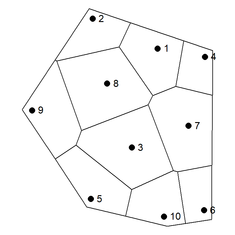
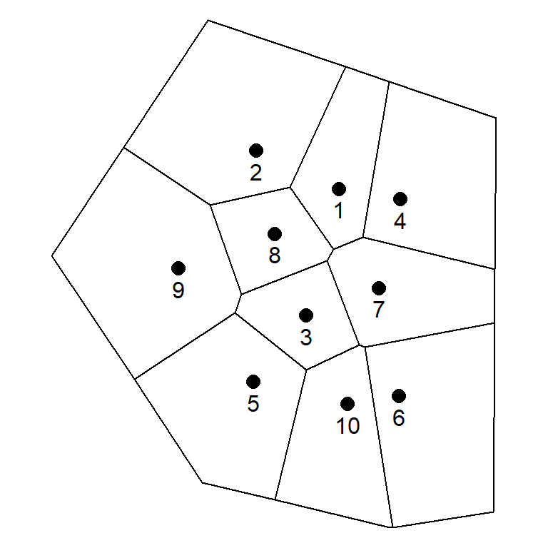
Figure 2: Thiessen polygons with 10% buffer zone (left plot) and 100% buffer zone (right plot).
Although it appears from Figure 2 that the internal polygons are smaller when using a larger value for the buffer, this is not the case. Areas of the internal polygons remain the same no matter the value used for the buffer. Areas of the outermost polygons, located along the hull boundary, increase with increasing buffer values. This is shown in Table 2, which provides the areas of the polygons shown for the 10 points in Figure 2. Areas for the internal polygons associated with points 3 and 8 are the same for both buffer values. Areas of the remaining polygons, located along the hull boundary, increased when the buffer value was changed from 10% to 100%. Because these areas increased, mass estimates for these outermost polygons also will increase and consequently, the total estimate of plume mass will increase. However, if the Thiessen tessellation is conducted using a consistent well network, the areas obtained for the Thiessen polygons remain constant over time. This eliminates the need to re-interpolate the groundwater concentration data for every sampling event. By eliminating the re-interpolation step, a baseline can be established that is relatively free of subjectivity inherent in other interpolation techniques, such as kriging.
# Load libraries
library(dplyr)
library(kableExtra)

# Get well ids
plocs_1 <- sapply(slot(sr1, "polygons"), slot, "ID")
plocs_2 <- sapply(slot(sr2, "polygons"), slot, "ID")

# Get areas
areas_1 <- sapply(slot(sr1, "polygons"), slot, "area") %>%
  bind_cols(Point = plocs_1) %>%
  rename(Area_10Per = ...1) %>%
  dplyr::select(Point, Area_10Per)

areas_2 <- sapply(slot(sr2, "polygons"), slot, "area") %>%
  bind_cols(Point = plocs_2) %>%
  rename(Area_100Per = ...1) %>%
  dplyr::select(Point, Area_100Per)

# Combine areas
areas <- areas_1 %>%
  left_join(areas_2, by = 'Point') %>%
  bind_rows(summarise_all(., ~if(is.numeric(.)) sum(.) else "Total")) %>%
  mutate_at(vars(- c(Point)), round, 0) %>%
  rename('Buffer 10%' = Area_10Per, 'Buffer 100%' = Area_100Per)

kbl(
  areas, align = 'crr',
  format.args = list(big.mark = ","),
  caption = 'Thiessen Polygon Areas', booktabs = T) %>%
  kable_classic_2(full_width = F, html_font = 'Cambria')
| Point | Buffer 10% | Buffer 100% |
|---|---|---|
| 1 | 2,730 | 6,033 |
| 2 | 1,930 | 14,243 |
| 3 | 4,476 | 4,476 |
| 4 | 1,433 | 10,756 |
| 5 | 2,590 | 11,139 |
| 6 | 1,518 | 12,309 |
| 7 | 3,921 | 7,452 |
| 8 | 4,617 | 4,617 |
| 9 | 2,924 | 14,596 |
| 10 | 2,166 | 7,951 |
| Total | 28,306 | 93,572 |
Thiessen polygons are an exact method of interpolation that assumes values at unsampled locations are equal to the value of the nearest sampled point. Unlike Thiessen polygons, kriging predicts the values at unsampled locations based on the degree of spatial dependence between sampled locations. This requires development of a semivariogram model that best fits the data to produce the optimum weights for interpolation. The variogram model parameters in kriging include a certain degree of subjectivity, which will influence the accuracy of interpolation. This subjectivity is absent in Thiessen polygons, however, if data are sparse and unevenly spaced, estimation using Thiessen polygons will be dominated by these sparsely located points.
General Procedure
The steps required to estimate total dissolved-phase mass and center-of-mass for each contaminant and time period are listed below.
Step 1. Establish a Consistent Monitoring Network. A consistent set of monitoring wells is required in order to detect changes in estimated dissolved-phase contaminant mass and the estimated center-of-mass through time. When selecting the well network it is important to consider the spatial distribution of potential locations and the contaminant history at these locations. A more densely populated well network may be advisable in highly contaminated areas to more accurately represent the contaminant mass in this area.
Step 2. Construct Thiessen Polygons Around Individual Monitoring Locations. Polygons are generated from the chosen monitoring locations and constrained to the defined area of analysis. The magnitude of the buffer zone applied should be chosen to reflect the density of monitoring locations within the polygon network (i.e., the buffer zone is smaller when monitoring locations in the network are more dense, and larger when monitoring locations are more sparse).
Step 3. Calculate the Area of Individual Thiessen Polygons. The areas of individual Thiessen polygons is calculated and then used to estimate contaminant mass and center-of-mass.
Step 4. Estimate Total Dissolved-Phase Contaminant Mass. The estimated mass of contamination in each polygon is calculated using the individual polygon areas, the average total porosity of the aquifer, and the average thickness of the aquifer. Calculate the total mass as the summation of the mass for each individual polygon (see equation 3).
Step 5. Estimate the Center-of-Mass. To estimate the center-of-mass, the coordinates of each polygon (i.e., the coordinates of the monitoring well that represents the polygon) are weighted by the calculated estimated mass of the polygon. Calculate the center-of-mass \((X_c, Y_c)\) as the summation of the weighted coordinates divided by the total dissolved mass (see equations 6 and 7).
If these steps are applied to multiple sampling events, a statistical trend analysis can be performed to document changes in the plume condition over time. Additionally, the change in the location of the center-of-mass can be plotted on a site base map to identify whether the dissolved-phase contaminant center-of-mass is advancing, stable, or receding.
Example Calculation
Tabulated results from an example calculation are shown below. In this example, the sample locations from Figure 2 will be used to estimate the total dissolved-phase mass and center-of-mass for a single monitoring event. The average total porosity and thickness of the aquifer are assumed to be 30% and 10 feet, respectively. Thiessen areas have been calculated using a buffer zone of 10% (see Table 1). Fabricated concentrations (in milligrams-per-liter) have been assigned to each sample location. For each sample location, the estimated mass of contamination and weighted weighted coordinates have been calculated. The total dissolved-phase mass is 74.5 kilograms (kg) and the coordinates of the center-of-mass are \(X_c\) = 114 and \(Y_c\) = 99.

The location of the center-of-mass for this sampling event is shown in Figure 3. Also shown in the figure are the sample point locations and the Thiessen polygons created from these sample points using a buffer zone of 10%. The polygons are color-coded by the dissolved-phase mass estimated for each polygon. The center-of-mass is located between sample points #3 and #8, which are associated with the highest estimates of contaminant mass (18.3 and 16.1 kg, respectively) as shown in the table above.
# Load libraries
library(ggplot2)
library(ggrepel)
library(RColorBrewer)

# Add concentrations to pts
Conc <- c(
  24, 15, 48, 26, 20,
  33, 34, 41, 23, 18
)

pts <- data.frame(pts, Conc)

# Set parameters
thick <- 10         # uniform aquifer thickness, in feet
por <- 0.30         # bulk porosity
CF <- 2.831685e-5   # conversion factor based on mg/L

# Merge areas with data file and calculate mass
pts_mass <- areas[-11, ] %>%
  select(Point, 'Buffer 10%') %>%
  rename(Area = 'Buffer 10%') %>%
  mutate(Point = as.numeric(Point)) %>%
  left_join(pts, by = c('Point' = 'id')) %>%
  mutate(
    Mass = Area * thick * por * Conc * CF,
    Xi   = x * Area * thick * por * Conc * CF,
    Yi   = y * Area * thick * por * Conc * CF
  )

# Calculate total mass and CoM
pts_com <- pts_mass %>%
  summarize(
  Mass  = sum(Mass),
  Xc = sum(Xi)/sum(Mass),
  Yc = sum(Yi)/sum(Mass)
)

# Create bins for coloring polygons
bins <- c(0, 4, 8, 12, 16, 20)
nint <- length(bins)
levells <- NULL
for (i in 1:(nint - 1)) {
  levells <- c(levells, paste(bins[i], "-", bins[i + 1]))
}

IDs <- sapply(slot(sr1, "polygons"), function(x) slot(x, "ID"))
df <- data.frame(rep(0, length(IDs)), row.names = IDs)
srDF <- SpatialPolygonsDataFrame(sr1, df)

# Save the data row.names into an explicit variable
srDF$rn <- row.names(srDF)

# Create concentration ranges for polygon colors
brks <- cut(pts_mass$Mass, breaks = bins, dig.lab = 9)
brks <- gsub(","," - ", brks, fixed = TRUE)
pts_mass$brks <- gsub("\\(|\\]", "", brks)  # reformat guide labels
pts_mass$brks <- factor(pts_mass$brks, levels = levells)

# Create new data where
newData <- merge(srDF@data, pts_mass[, c('Point', 'brks')],
                 by.x = "rn", by.y =  "Point")

# Sort by newData by srDF rownames
newData <- newData[match(row.names(srDF),newData$rn), ]

# Add new data to srDF
srDF@data <- newData

# Create files for using ggplot polygons
srDF@data$id = rownames(srDF@data)
srDF.points = fortify(srDF, region = "id")
srDF.df = plyr::join(srDF.points, srDF@data, by = "id")

# Create plot
p <-  ggplot() +
    geom_polygon(data = srDF.df, aes(x = long, y = lat, group = group,
                 fill = brks), alpha = 0.4) +
    geom_path(data = srDF.df, aes(x = long, y = lat, group = group),
              color = 'grey40', alpha = 1) +
    geom_point(data = pts, aes(x = x, y = y),
               pch = 16, size = 3, color = 'black') +
    geom_point(data = pts_com, aes(x = Xc, y = Yc),
               pch = '+', size = 10, color = 'blue') +
    geom_text_repel(data = pts, aes(x = x, y = y, label = id),
                    size = 4, segment.size = 0.3,
                    nudge_x = 0, nudge_y = -0.3,
                    point.padding = unit(0.01, "lines")) +
    annotate('text', label = 'Center-of-Mass', x = 114, y = 90,
             size = 4, color = 'blue', fontface = 2) +
    labs(title = NULL,
         subtitle = NULL,
         x = 'X Coordinate',
         y = 'Y Coordinate') +
    scale_fill_brewer(name = 'Mass (kg)',
                      palette = "YlOrRd",
                      drop   = FALSE) +
    coord_fixed() +
    theme_void()
p
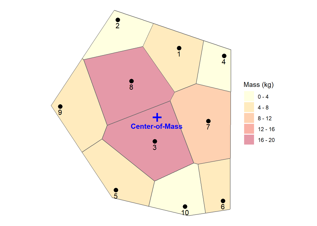
Figure 3: Sample points, Thiessen polygons, and location of center-of-mass.
References
Air Force Center for Environmental Excellence (AFCEE). 2002. Monitoring and Remediation Optimization System (MAROS): Software Version 2.0 User’s Guide. Brooks City-Base, Texas.
Aris, R. 1956. On the dispersion of a solute in a fluid flowing through a tube. Proc. R. Soc. London, Ser. A 235, 67-77.
Brassel, K.E. and D. Reif. 1979. A procedure to generate Thiessen polygons. Geographical Analysis. 11, 290-303.
Brauner, J.S., D.C. Downey, and R. Miller. 2010. Using Advanced Analysis Approaches to Complete Long-Term Evaluations of Natural Attenuation Processes on the Remediation of Dissolved Chlorinated Solvent Contamination. Prepared for the Strategic Environmental Research and Development Program, SERDP Project ER-1348. October.
Chow, V.T., D.R. Maidment, and L.W. Mays. 1988. Applied Hydrology. New York, McGraw-Hill.
Dupont, R.R. 1998. Monitoring and Assessment of In-Situ Biocontainment of Petroleum Contaminated Ground-Water Plumes. Prepared for the National Exposure Research Laboratory, Office of Research and Development, U.S. Environmental Protection Agency, EPA/600/R-98/020. February.
Freyberg, D.L. 1986. A natural gradient experiment on solute transport in a sand aquifer 2. Spatial moments and the advection and dispersion of non-reactive tracers. Water Resources Research 22, 2031-2046.
Gilbert, R.O. 1987. Statistical Methods for Environmental Pollution Monitoring. Wiley, New York.
Gorder, K., Hall, B.L., C. Holbert, and S. Snelgrove. 2006. Performance Monitoring for Remedial Process Optimization at Hill AFB Operable Unit 2. Proceedings of the Fifth International Conference on Remediation of Chlorinated and Recalcitrant Compounds, Monterey, California, May 22-25.
Gorder, K. and Holbert, C. 2010. Thiessen Area and Mass Calculator for Assessment of Plume Dynamics. Proceedings of the Seventh International Conference on Remediation of Chlorinated and Recalcitrant Compounds, Monterey, California, May 24-27.
Guven O., F.J. Molz, and J.G. Melville 1984. An analysis of dispersion in a stratified aquifer. Water Resour Res. 20, 1337-1354.
Hyam, M. and R.R. Dupont. 2001. Groundwater and Soil Remediation: Process Design and Cost Estimating of Proven Technologies. Reston, ASCE Press.
Kendall, M.G. 1975. Rank Correlation Techniques, 4th edition. Charles Griffen. London.
Mann, H.B. 1945. Nonparametric Tests Against Trend. Econometrica 13, 245-259.
Marle, C., P. Simandoux, J. Pacsirszky, and C. Caulier. 1967. Study of the displacement of miscible fluids in a porous stratified medium. Rev. Inst. Franc. petroleum 22, 272-294.
Ripley, B.D. 2004. Spatial Statistics. Wiley-Interscience, New York.
Sibson, R. 1980. The Dirichlet tessellation as an aid in data analysis. Scandinavian Journal of Statistics 7, 14-20.
United States Environmental Protection Agency (EPA). 2009. Statistical Analysis of Groundwater Monitoring Data at RCRA Facilities: Unified Guidance. EPA-530-R-09-007. Office of Resource Conservation and Recovery, U.S. Environmental Protection Agency. March.
- Posted on:
- April 2, 2022
- Length:
- 25 minute read, 5140 words
- See Also: