Multivariate Analysis Using Data With Non-detects
By Charles Holbert, Jacobs
September 2, 2020
Introduction
Multivariate statistical methods provide a means of exploring complex data sets for patterns and relationships from which hypotheses can be generated and subsequently tested. They reflect more accurately the true multidimensional, multivariate nature of natural environmental systems. Multivariate methods are used extensively in environmental science. They are used to help ecologists discover structure and provide a relatively objective summary of the primary features of a complex data set for easier comprehension. In environmental monitoring, multivariate statistical techniques are used to evaluate and assist with understanding anthropogenic changes to the environment. For instance, multivariate methods are used to explore patterns among contaminants, indicating which contaminants are routinely found together. Combined with explanatory variables, these patterns may provide insight into processes affecting spatial distribution of contaminants within the environment.
Helsel (2012) summarizes multivariate methods that can be used to analyze data containing censored (nondetect) observations, including issues that arise when improperly managing non-detects. Ignoring variables with non-detects or substituting proxy values, such as some fraction of the detection or reporting limit (RL), for non-detects can be eliminated by using multivariate approaches that capture the information in the pattern of detected values along with the pattern in the frequency of data below each censoring limit.
The objective of this factsheet is to focus on how to manage non-detects when applying multivariate procedures to investigate (dis)similarities among data objects based on a set of descriptors. These procedures include binary methods, ordinal nonparametric methods, and methods that operate on data scores while adjusting for frequencies of censored observations. While the first two methods are valid for one RL, or censoring at the highest RL, the last method can be used with data containing multiple RLs (Helsel 2012).
Data
The data used in this factsheet contain concentrations for variants of the toxic chemical compounds DDT, DDE, and DDD found in fish. The fish are classified into one of two age groups, Young or Mature. The objective is to test whether the pattern of chemicals differs between the various sites, and between Young and Mature age fish.
The structure of the data is shown below. The data consist of 7 variables with 192 observations. The variables include the following:
- Site
- Date, decimal format
- Analyte
- Detected, Yes(Y) or No (n)
- Result
- Flag, for data qualifiers
- Age, Young or Mature
# Load libraries
library(dplyr)
library(reshape2)
library(ggplot2)
library(ggrepel)
library(vegan)
library(MASS)
library(FactoMineR)
library(factoextra)
library(RColorBrewer)
library(colorspace)
library(dendextend)
library(EnvStats)

# Set seed
set.seed(10)

# Read data in comma-delimited file
datin <- read.csv('./data/FishDDT.csv', header = T)
str(datin)
## 'data.frame':	192 obs. of  7 variables:
##  $ Site    : int  1 2 3 4 5 6 7 8 9 10 ...
##  $ Date    : num  1996 1990 1994 2002 2000 ...
##  $ Analyte : chr  "opDDD" "opDDD" "opDDD" "opDDD" ...
##  $ Detected: chr  "N" "N" "Y" "N" ...
##  $ Result  : num  5 5 5.3 2 2 2 3.1 2 3.1 5.1 ...
##  $ Flag    : chr  "U" "U" "" "U" ...
##  $ Age     : chr  "Young" "Mature" "Mature" "Mature" ...
Multivariate Methods
Measuring the association between objects or descriptors is generally the first step in the numerical analysis of multivariate data. The most common approach to assess resemblance is to first condense all (or the relevant part of) the information available in the data into a square matrix of association among the objects or descriptors. Ths is referrred to as a resemblance matrix, a concise summary of the similarities or distances between all possible pairs of the data (Wildi 2010). A triangular-shaped matrix results from computing numerical measures of similarity (or conversely, distance) between all pairs of data. Resemblance measures include correlation coefficients such as Pearson’s r, Spearman’s rho, or Kendall’s tau; Euclidean distances between points in multidimensional space (where small distances indicate similar sites); or more specialized measures from the biological sciences. Resemblance measures particularly suited to censored data are listed below. A more complete discussion of resemblance measures is given in Zuur et al. (2007) and Clarke and Warwick (2001).
| Resemblance Measure | Type of Data | Resulting Procedures |
|---|---|---|
| Simple matching | Presence/absence | Binomial methods |
| Euclidean distance | Ranks of data | Ordinal methods |
| Euclidean distance | u-Scores | Wilcoxon-type methods |
The following three multivariate methods for analyzing data containing non-detects will be presented:
- Binary methods based on detects/non-detects using a matching coefficient
- Euclidean distances based on data ranks
- Euclidean distances based on u-scores
Binary Method - Symmetrical Matching Coefficient
A simple procedure to employ multivariate methods for censored data is to recensor data into two groups, below versus greater than or equal to the highest RL. A binary multivariate resemblance matrix can then be computed. Several similarity coefficients are used in the biological sciences for presence/absence (0/1) data.
Distance or similarity measures are essential in solving many pattern recognition problems such as classification and clustering. The simplest way for comparing the similarity and diversity of sample sets is the matching coefficient (Sokal and Michener 1958). The matching coefficient does not impose any weights on the data but represents the number of shared index terms. For a given variable, it assigns the value 1 in case of a match and the value 0 otherwise. The matching coefficient ($S_{ij}$) for a resemblance matrix is given by:
$$S_{ij} = \frac{(a + d)}{(a + b + c + d)}$$
where a equals the number of joint occurrences of a 1, d equals the joint occurrences of a 0, and b and c are mismatches where one site in the pair has a presence and one an absence of a detection above the highest RL. If a high value is switched from the designation of a 0 to that of a 1, a and d switch places, as do b and c, but the computed matching coefficient stays the same (Helsel 2012).
Descriptive statistics of the fish data using the Kaplan-Meier (KM) product-limit estimator (Kaplan and Meier 1958) for non-detects is shown below. The KM method is a nonparametric method designed to incorporate data with multiple censoring levels and does not require an assumed distribution. Originally, this method was developed for analysis of right censored survival data where the KM estimator is an estimate of the survival curve, a complement of the cumulative distribution function. The KM method estimates a cumulative distribution function that indicates the probability for an observation to be at or below a reported concentration. The estimated cumulative distribution function is a step function that jumps up at each uncensored value and is flat between uncensored values.
# Review a summary of the data by group
dat <- datin %>%
  mutate(Censored = ifelse(Detected == 'N', TRUE, FALSE))

# Calcuate summary statistics
cdat <- dat %>%
  group_by(Age) %>%
  summarize(
    Obs     = length(Result),
    Dets    = length(Result[Detected == 'Y']),
    NDs     = length(Result[Detected == 'N']),
    Min.ND  = tryCatch(min(Result[Detected == 'N'], na.rm = T),
                       warning = function(e) NA),
    Max.ND  = tryCatch(max(Result[Detected == 'N'], na.rm = T),
                       warning = function(e) NA),
    Min.Det = tryCatch(min(Result[Detected == 'Y'], na.rm = T),
                       warning = function(e) NA),
    Max.Det = tryCatch(max(Result[Detected == 'Y'], na.rm = T),
                       warning = function(e) NA),
    Mean   = tryCatch(enparCensored(Result, CENSORED)$parameters['mean'],
                      error = function(e) mean(Result, na.rm = T)),
    Median  = tryCatch(median(ppointsCensored(Result, Censored,
                              prob.method = 'kaplan-meier')$Order.Statistics),
                       error = function(e) median(Result, na.rm = T)),
    SD      = tryCatch(enparCensored(Result, Censored)$parameters['sd'],
                       error = function(e) sd(Result, na.rm = T))
  ) %>%
  ungroup %>%
  mutate_at(4:11, round, 1) %>%
  data.frame()

knitr::kable(cdat, align = "lcccccccccc",
             col.names = gsub("[.]", " ", names(cdat)),
             caption = "Descriptive Statistics")
Table: Table 1: Descriptive Statistics
| Age | Obs | Dets | NDs | Min ND | Max ND | Min Det | Max Det | Mean | Median | SD |
|---|---|---|---|---|---|---|---|---|---|---|
| Mature | 156 | 99 | 57 | 2 | 5 | 3.1 | 250 | 24.8 | 6.7 | 44.4 |
| Young | 36 | 5 | 31 | 2 | 5 | 14.0 | 23 | 4.5 | 2.0 | 5.4 |
The highest reporting limit in the data is 5. For this first method, the data will be coded as a 1 for concentrations greater than or equal to 5, and a 0 for concentrations less than 5. Similarities will be calculated using 1.00001 - \(S_{ij}\), where a very small constant is added to ensure no similarities are exactly zero.
Nonmetric Multidimensional Scaling
Nonmetric multidimensional scaling (NMDS) (Kruskal 1964; Cox and Cox 2001; Zuur et al. 2007) can be used to create a plot of the age similarities between the two groups of fish. NMDS plots the distances between points in the same rank order as distances (or similarities) in the resemblance matrix. The goal of NMDS is to collapse information from multiple dimensions (e.g, from multiple communities, sites, etc.) into just a few, so that they can be visualized and interpreted. NMDS iteratively manipulates coordinates of pairs of observations so they fit as closely as possible to measured object similarities. NMDS is similar to principal component analysis (PCA) in that it provides a representation of relationships between data objects in a reduced number of dimensions. Because NMDS is a rank-based approach, meaning that the original distance data is substituted with ranks, it is generally more robust to data which do not have an identifiable distribution.
As in any data analysis problem, an expression is needed to express how well a particular set of data are represented by the model that the analysis imposes. In the case of NMDS, a stress parameter is computed to measure the lack of fit between object distances in the NMDS ordination space and the calculated dissimilarities among objects. The NMDS algorithm iteratively repositions the objects in the ordination space to minimize the stress function. The stress function is given as following:
$$stress = \frac{\sum{(d_{ij} - \hat{d_{ij}})^2}}{\sum{d_{ij}^2}}$$
where \(\hat{d_{ij}}\) is the predicted distance based on the NMDS model. NMDS models with stress values near zero are optimal. As a general rule, solutions with higher stress values (usually above 0.20) should be interpreted with caution; stress values less than 0.1 are considered generally acceptable (Kruskal 1964). In reality, acceptable values of stress depends on the quality of the distance matrix and the number of objects in that matrix.
On a NMDS plot, objects that are closer to one another are likely to be more similar than those further apart. Tight clusters of points that are well-separated from other clusters may indicate sub-populations in the data. However, it’s important to note that the scale of the axes is arbitrary as is the orientation of the plot.
The NMDS plot for the fish data using the binary method and matching coefficients is shown below.
# Funtion for suppressing output
quiet <- function(x) {
  sink(tempfile())
  on.exit(sink())
  invisible(force(x))
}

# Code to 0 for concentrations less than or equal to 5 and 1 for concentrations
# greater than 5.
dat <- datin
dat <- within(dat, {
    Result2 = ifelse(Result <= 5, 0, 1)
})

# Use dcast from reshape to change from long to wide format
datw <- dcast(dat, Site + Date + Age ~ Analyte, value.var = 'Result2')
datw$Age <- factor(datw$Age)

# Define similarities uisng the designdist command, which computes a user-
# defined distance matrix, which here is 1?similarity (with a very small
# constant added to ensure no distances are exactly zero).
ddt.symm <- designdist(
  datw[, 4:9],
  method = "1.00001-((a+d)/(a+b+c+d))",
  terms = "binary", abcd = TRUE,
  alphagamma = FALSE, name = "symm"
)

# Run the metaMDS command from the vegan package to generate an NMDS plot
ddt.mds <- quiet(
  metaMDS(
    ddt.symm,
    zerodist = "add",
    autotransform = FALSE,
    trymax = 20
  )
)

# Extract NMDS scores (x and y coordinates)
data.scores <- as.data.frame(scores(ddt.mds))
datwMDS <- cbind(datw, data.scores)

# Plot ordination
xmin <- min(datwMDS$NMDS1)
ymin <- min(datwMDS$NMDS2)
pos <- position_jitter(width = 0.1, seed = 2)
p <- ggplot(datwMDS, aes(NMDS1, NMDS2, color = Age)) +
  geom_jitter(position = pos, shape = 16, size = 3) +
#  stat_ellipse(type = 't', size = 1) +   #95% confidence interval ellipses
  geom_text_repel(data = datwMDS, aes(NMDS1, NMDS2, label = Site),
                  position = pos,
                  size = 3, segment.size = 0.1,
                  color = "black",
                  box.padding = unit(0.2, "lines"),
                  point.padding = unit(0.2, "lines")) +
  labs(title = "NMDS Plot - Binary Method with Matching Coefficient",
       subtitle = "DDT and Related Compounds in Fish" ) +
  scale_color_brewer(palette = "Set1") +
  annotate("text", x = xmin, y = ymin, hjust = 0,
           label = paste('2D Stress =', round(ddt.mds$stress, 3))) +
  theme_minimal() +
  theme(legend.box = "vertical", legend.position = "bottom")
p
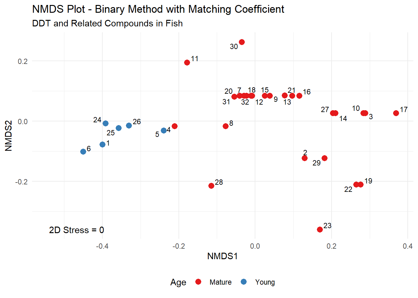
Sites 1, 5, and 24 through 26 all have nondetect (below 5) concentrations for all compounds except ppDDE. These five sites are clustered in the left portion of the NMDS plot. Site 6 has non-detects for all six compounds, and is located just to the left of the other five sites. These six sites are associated with fish of a Young age. Sites 4 and 8 have detected concentrations for ppDDE and ppDDT, and plot to the right of the Young age group. Sites with detections of more than two compounds are located on the right side of the NMDS plot and are associated with fish of a Mature age.
Analysis of Similarity
To test the hypothesis of no difference in the pattern of DDT and related compound concentrations between the two groups, the nonparametric Analysis of Similarity (ANOSIM) test (Clarke 1999) can be employed. The ANOSIM test has some similarity to an analysis of variance (ANOVA) hypothesis test, however, it is used to evaluate a dissimilarity matrix rather than raw data. Because raw dissimilarities are often ranked prior to performing an ANOSIM, the test is aligned with the NMDS procedure. Together, the dimension reduction and visualization capacities of NMDS and the hypothesis testing offered by ANOSIM are complementary approaches in evaluating nonparametric multivariate data.
datw.ano <- with(datw, anosim(ddt.symm, Age))
summary(datw.ano)
##
## Call:
## anosim(x = ddt.symm, grouping = Age)
## Dissimilarity: symm
##
## ANOSIM statistic R: 0.6876
##       Significance: 0.001
##
## Permutation: free
## Number of permutations: 999
##
## Upper quantiles of permutations (null model):
##   90%   95% 97.5%   99%
## 0.152 0.205 0.245 0.315
##
## Dissimilarity ranks between and within classes:
##            0%   25%   50%   75%  100%   N
## Between 153.0 305.5 428.0 428.0 495.5 156
## Mature   39.5 153.0 153.0 305.5 483.5 325
## Young    39.5  39.5  39.5 153.0 153.0  15
plot(datw.ano)
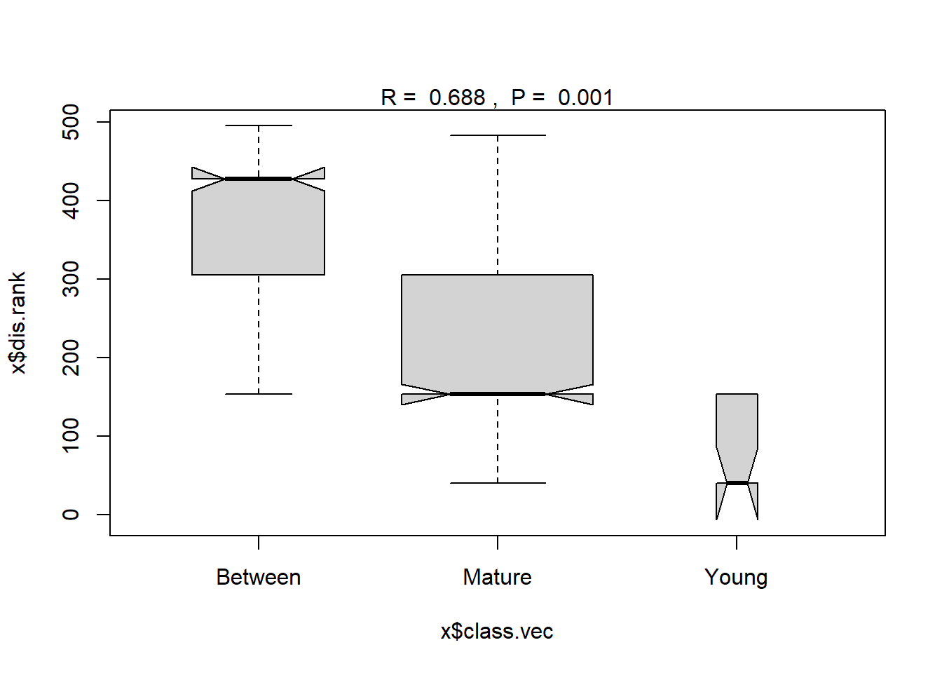
The resulting probability, or p-value, for the ANOSIM test is 0.001. Based on a significance level of 0.05, the null hypothesis that the patterns of the six chemicals is the same in both Young and Mature age fish is rejected; the two groups are determined to have different patterns of DDT and metabolites.
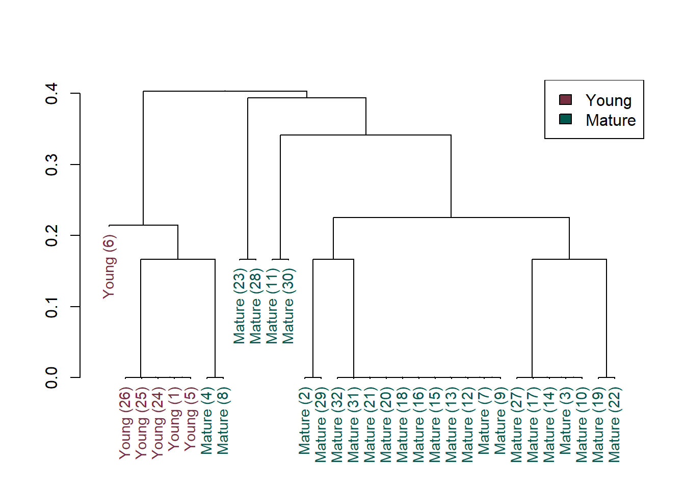
Cluster Analysis
Cluster analysis can be used to extract information on data groupings using a resemblance matrix for binary data. The distance matrix created above for the binary detect/nondetect fish data can be clustered and the dendrogram plotted. Sites that are more similar to one another are placed into the same cluster whereas sites that are less similar to one another are placed in different clusters.
ddt.clust <- hclust(ddt.symm, "average")

# Create dendrogram with colored labels by age using dendextend
datw_age <- rev(levels(datw[, 3]))
dend <- as.dendrogram(ddt.clust)

# Manually match the labels, as much as possible, to the real age
labels_colors(dend) <-
   rainbow_hcl(2, c = 45, l = 30)[sort_levels_values(
      as.numeric(datw[, 3])[order.dendrogram(dend)]
   )]

# Add age to the labels
labels(dend) <- paste(
  as.character(datw[,3])[order.dendrogram(dend)],
  " (", labels(dend), ")", sep = ""
)

# Hang the dendrogram a bit
dend <- hang.dendrogram(dend, hang_height = 0.001)

# Reduce the size of the labels
dend <- set(dend, "labels_cex", 0.9)

# Make the plot
plot(dend, nodePar = list(cex = .007))
legend("topright", legend = datw_age, fill = rainbow_hcl(2, c = 45, l = 30))
Principal Component Analysis
PCA can be used for a combined inspection of the pattern of sites and pattern of compounds using a biplot. PCA finds the two primary linear directions through multidimensional space that best describe the variability of the data. In essence, these two components maximize the spread of the data on the plot in comparison to any other viewpoint. Biplots are plots of the projections of the sites and compounds onto the first two principal components. Biplots present a two-dimensional slice through multivariate space. A biplot is more restrictive than NMDS in that it assumes linear relationships between variables. The benefit of a biplot over NMDS is that it produces axes that are linear combinations of the original variables.
# Perform PCA
ddt.pca <- princomp(datw[, 4:9], cor = TRUE)

# Create biplot
p <- fviz_pca_biplot(
       ddt.pca, axes = c(1, 2),
       mean.point = FALSE,
       geom.ind = "point",
       pointsize = 3,
       col.ind = datw$Age, habillage = datw$Age,
       label = "var", repel = TRUE,
       title = "PCA Biplot - Binary Method with Matching Coefficient",
       subtitle = "DDT and Related Compounds in Fish",
       caption = "") +
     theme_bw() +
     scale_color_brewer(palette = "Set1") +
     theme(legend.box = "vertical", legend.position = "bottom")
p
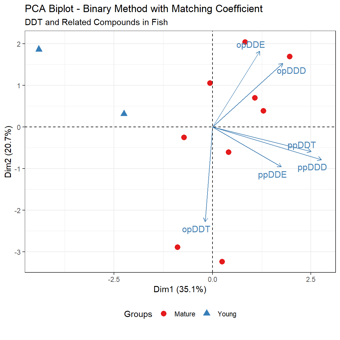
In the biplot shown above, principal component (PC) 1 (referred to as DIM 1 in the plot) is a contrast between higher concentrations of pp- isomers to the right, and low concentrations to the left. This is evident from the direction the ppDDT, ppDDD, and ppDDE vectors are pointing - vectors on a biplot point toward the direction of higher values. The sites with Young age fish are to the left, showing lower concentrations of the six compounds. PC 2 (referred to as DIM 2) is based on the op- isomers, with higher values of opDDT toward the bottom (low PC 2 values) and higher values of opDDD and opDDE generally toward the top (high values of PC 2). This second PC splits the patterns in the Mature age fish by whether opDDT or its metabolites are more often present in concentrations above the RL.
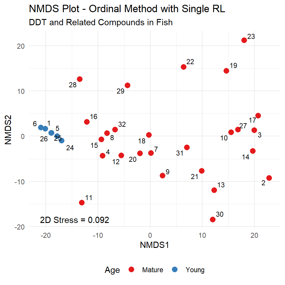
Ordinal Method - One Reporting Limit
Additional information is contained in the relative order (ranks or percentiles) of values above the highest RL. Ordinal nonparametric methods capture this additional information by assigning unique ranks to data at and above that limit, while ranks of all data below the highest limit are tied with one another. Many nonparametric methods can be thought of as tests on the average rank (Conover and Iman 1981). For example, the Kruskal-Wallis test can be approximated by whether the average rank is similar or different in each of k groups.
For the fish data, all values within each compound class originally reported as below the highest RL of 5 will have the same average rank, which is below the ranks of the detected concentrations above 5 for that compound. The NMDS plot for the ranked DDT fish data using the Euclidean distance measure is shown below. The Young and Mature age groups of fish are located on different areas of the plot, illustrating their different chemical signatures.
# Assign the value of 5 to concentrations less than or equal to 5 and then rank
# concentrations within each group
dat <- datin %>%
  mutate(Result = ifelse(Result <= 5, 5, Result)) %>%
  group_by(Analyte) %>%
  mutate(Rank.Result = rank(Result, ties.method = "average")) %>%
  ungroup

# Use dcast from reshape to change from long to wide format
datw <- dcast(dat, Site + Date + Age ~ Analyte, value.var = 'Rank.Result')

# Run the metaMDS command from the vegan package to generate an NMDS plot
f.mds <- quiet(
  metaMDS(
    datw[, 4:9],
    distance = "euclidean",
    zerodist = "add",
    autotransform = FALSE,
    trymax = 20
  )
)

# Extract NMDS scores (x and y coordinates)
data.scores = as.data.frame(scores(f.mds))
datwMDS <- cbind(datw, data.scores)

# Plot ordination
xmin <- min(datwMDS$NMDS1)
ymin <- min(datwMDS$NMDS2)
pos <- position_jitter(width = 0.1, seed = 2)
p <- ggplot(datwMDS, aes(NMDS1, NMDS2, color = Age)) +
  geom_jitter(position = pos, shape = 16, size = 3) +
#  stat_ellipse(type = 't', size = 1) +   #95% confidence interval ellipses
  geom_text_repel(data = datwMDS, aes(NMDS1, NMDS2, label = Site),
                  position = pos,
                  size = 3, segment.size = 0.1,
                  color = "black",
                  box.padding = unit(0.2, "lines"),
                  point.padding = unit(0.2, "lines")) +
  labs(title = "NMDS Plot - Ordinal Method with Single RL",
       subtitle = "DDT and Related Compounds in Fish" ) +
  scale_color_brewer(palette = "Set1") +
  annotate("text", x = xmin, y = ymin, hjust = 0,
           label = paste('2D Stress =', round(f.mds$stress, 3))) +
  theme_minimal() +
  theme(legend.box = "vertical", legend.position = "bottom")
p
Seriation Test
The test of seriation (Clark et al. 1993; Clarke and Warwick 2001) can be used to investigate whether concentrations in the Mature age fish are changing over time. The term seriation describes a consistent change in multivariate pattern along an axis of one external explanatory variable not used to construct the multivariate resemblance matrix (Helsel 2012). Here the external variable is Date, a time sequence. As a nonparametric test, a change in pattern is tested against the ranks of the explanatory variable, and so is applicable to any ordinal or continuous variable. The test is in essence a multivariate analog of the popular univariate Mann-Kendall test for trend.
The test of seriation is computed by constructing an aggregate rank correlation coefficient such as Kendall’s tau between each element of two triangular matrices (Helsel 2012). Two points close together in time have a small rank, while comparisons between an early point and late point will have larger rank distance. If there is a correlation between the resemblance pattern and the pattern of rank distances along the explanatory axis, the null hypothesis of no seriation is rejected and a significant association between resemblance pattern and explanatory variable is established. The test for seriation is one of a class of tests called Mantel tests. The Mantel test (Mantel 1967) is used to calculate correlations between corresponding positions of two (dis)similarity or distance matrices derived from either univariate or multivariate data.
The resulting p-value for the seriation test is 0.001, indicating that concentrations of DDT and the related compounds in the Mature age fish are changing over time.
mat <- subset(datw, Age == "Mature")
time.dist <- dist(mat[, 2], method = "manhattan")
ddt.dist <- dist(mat[, 4:9], method = "euclidean")
seriation <- mantel(time.dist, ddt.dist, method = "kendall")
seriation
##
## Mantel statistic based on Kendall's rank correlation tau
##
## Call:
## mantel(xdis = time.dist, ydis = ddt.dist, method = "kendall")
##
## Mantel statistic r: 0.4889
##       Significance: 0.001
##
## Upper quantiles of permutations (null model):
##    90%    95%  97.5%    99%
## 0.0596 0.0793 0.0970 0.1183
## Permutation: free
## Number of permutations: 999
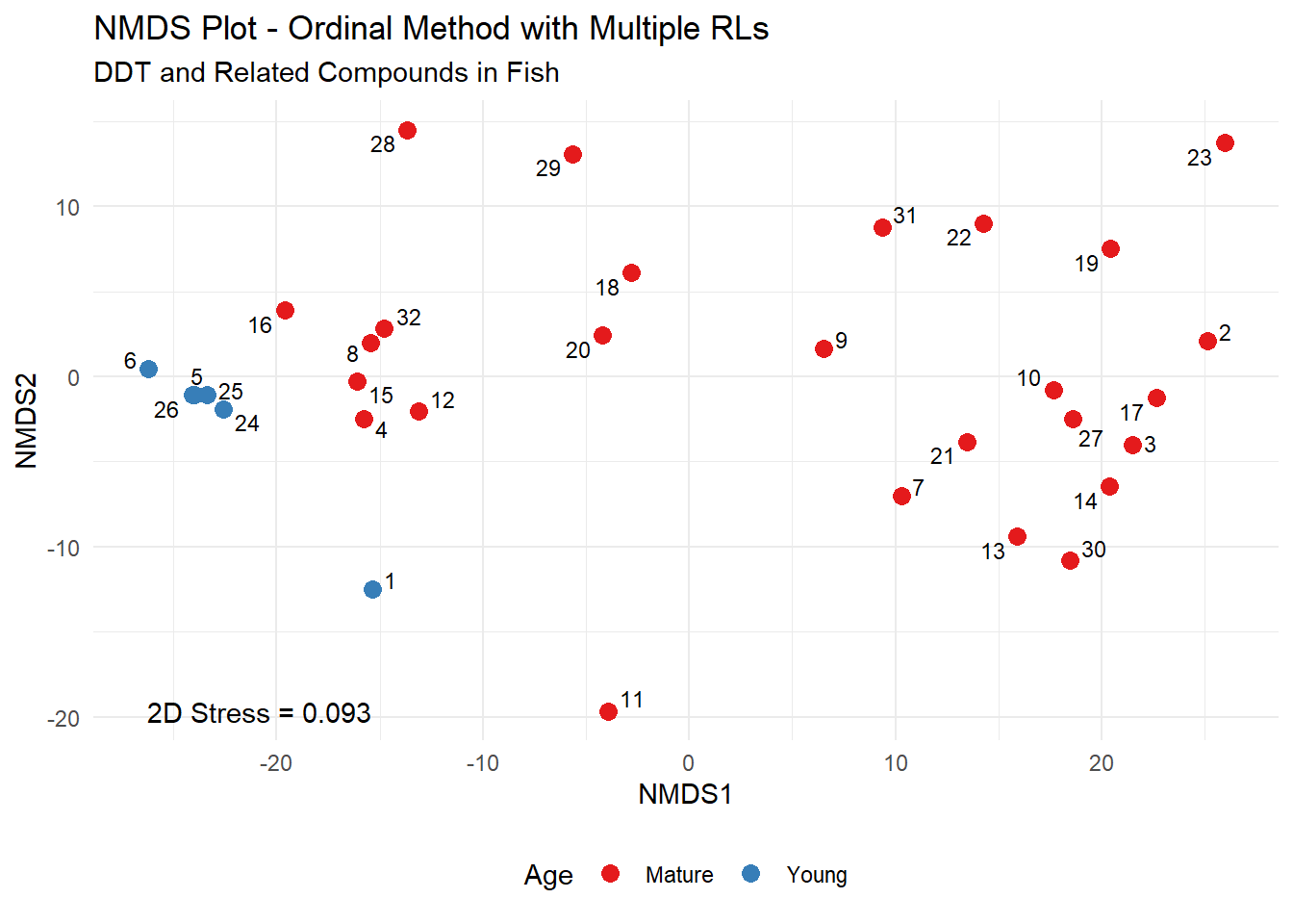
Ordinal Method - Multiple Reporting Limits
One of the simplest scoring statistics is the u-score. The u-score forms the basis for the Mann-Whitney test, and is related to Kendall’s tau and other nonparametric methods. The u-score is the sum of the algebraic sign of differences comparing the ith observation to all other observations within the same variable:
$$u_{i} = \sum_{i\neq k}sign(x_{i} - x_{k})$$
For the fish data, u-scores (and their ranks) were constructed variable by variable. Using a Euclidean distance measure on the u-scores or their ranks, NMDS, clustering, PCA, and other procedures can be applied to find and illustrate patterns in the data. Similar in concept to what was done after censoring at the highest RL, the difference now is that the scoring process accommodates censoring at multiple RLs. The corresponding NMDS plot conducted on the ranks of the u-scores is shown below. Similar to the previous results, the Young and Mature age groups of fish are located on different areas of the plot, illustrating their different chemical signatures.
uscore <- function(y, ind, rnk = T){

  n <- length(y)
  ylo <- (1 - ind) * y
  yadj <- y - (sign(y - ylo) * 0.001 * y)
  overlap <- y      # sets correct dimensions
  Score <- overlap  # sets correct dimensions

  for (j in 1:n) {
    for (i in 1:n ) {
      overlap[i] <- sign(sign(yadj[i] - ylo[j]) + sign(ylo[i] - yadj[j]))
    }
    Score[j] <- -1 * sum(overlap) 	# -1 so that low values = low scores
  }

  Urank <- rank(Score)

  if (rnk) {
    uscore <- rank(Score)
  } else {
    uscore = Score
  }
}

# Get uscores
dat <- datin %>%
  mutate(Censored = ifelse(Detected == 'N', TRUE, FALSE)) %>%
  group_by(Analyte) %>%
  mutate(Score = uscore(Result, Censored, rnk = T)) %>%
  ungroup

# Use dcast from reshape to change from long to wide format
datw <- dcast(dat, Site + Date + Age ~ Analyte, value.var = 'Score')
datw$Age <- factor(datw$Age)

# Run the metaMDS command from the vegan package to generate an NMDS plot
u.mds <- quiet(
  metaMDS(
    datw[, 4:9],
    distance = "euclidean",
    zerodist = "add",
    autotransform = FALSE,
    trymax = 20
  )
)

# Extract NMDS scores (x and y coordinates)
data.scores = as.data.frame(scores(u.mds))
datwMDS <- cbind(datw, data.scores)

# Plot ordination
xmin <- min(datwMDS$NMDS1)
ymin <- min(datwMDS$NMDS2)
pos <- position_jitter(width = 0.1, seed = 2)
p <- ggplot(datwMDS, aes(NMDS1, NMDS2, color = Age)) +
  geom_jitter(position = pos, shape = 16, size = 3) +
#  stat_ellipse(type = 't', size = 1) +   #95% confidence interval ellipses
  geom_text_repel(data = datwMDS, aes(NMDS1, NMDS2, label = Site),
                  position = pos,
                  size = 3, segment.size = 0.1,
                  color = "black",
                  box.padding = unit(0.2, "lines"),
                  point.padding = unit(0.2, "lines")) +
  labs(title = "NMDS Plot - Ordinal Method with Multiple RLs",
       subtitle = "DDT and Related Compounds in Fish" ) +
  scale_color_brewer(palette = "Set1") +
  annotate("text", x = xmin, y = ymin, hjust = 0,
           label = paste('2D Stress =', round(u.mds$stress, 3))) +
  theme_minimal() +
  theme(legend.box = "vertical", legend.position = "bottom")
p
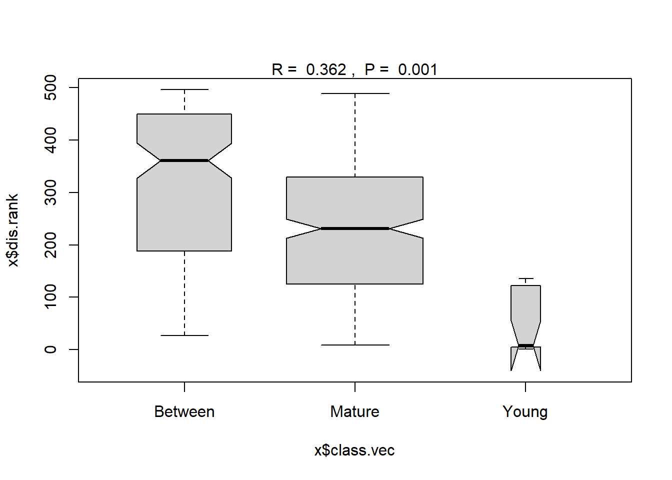
Results of ANOSIM to test the hypothesis of no difference in concentrations of DDT and the related compounds between the Young and Mature age fish using the ranks of the u-scores is provided below. The resulting p-value for the ANOSIM test is 0.001, indicating a statistically significant difference in concentrations between the Young and Mature age fish.
datw.ano <- with(datw,
  anosim(datw[, 4:9], Age, distance = "euclidean")
)
summary(datw.ano)
##
## Call:
## anosim(x = datw[, 4:9], grouping = Age, distance = "euclidean")
## Dissimilarity: euclidean
##
## ANOSIM statistic R: 0.362
##       Significance: 0.001
##
## Permutation: free
## Number of permutations: 999
##
## Upper quantiles of permutations (null model):
##    90%    95%  97.5%    99%
## 0.0904 0.1179 0.1486 0.1837
##
## Dissimilarity ranks between and within classes:
##         0%    25%   50%     75% 100%   N
## Between 27 189.50 361.0 449.125  496 156
## Mature   9 125.00 231.0 329.000  489 325
## Young    1   4.75   7.5 121.750  136  15
plot(datw.ano)
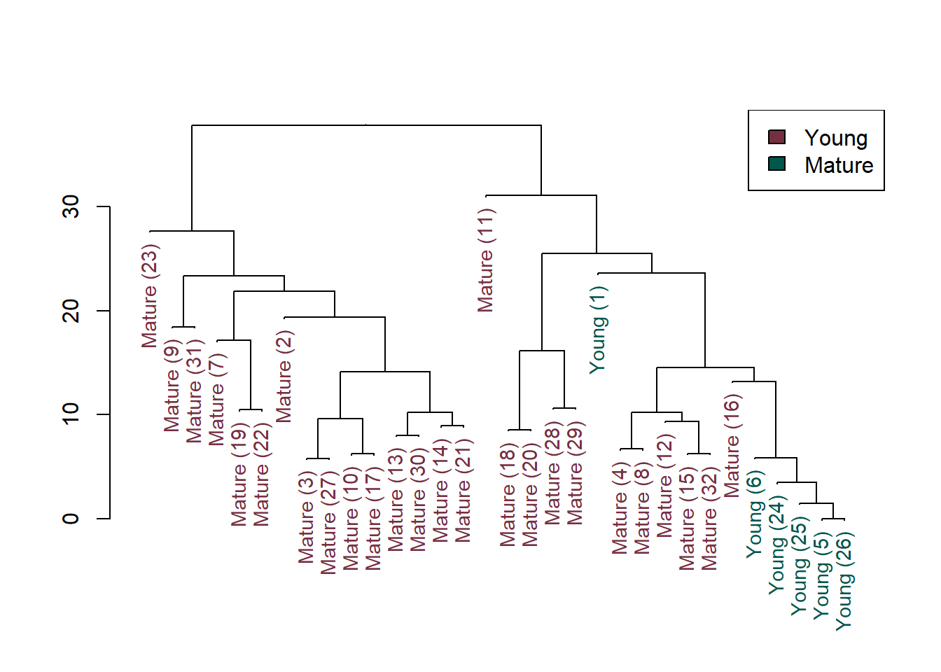
A dendrogram for cluster analysis performed on the ranks of the u-scores is plotted below. Compared to clustering using the binary data, clustering using the u-score data shows that several clusters are significantly different from one another. Site 1 is isolated from the other clusters, as is Site 11. Sites 18, 20, 28, and 29 cluster together and differ from sites further to the right on the dendrogram. The Young age fish are clustered togther except for Site 1, which has higher RLs than the other Young age fish.
Although valuable information is contained in the relative order of values above the highest RL, increased numerical detail provided by the multiple RL procedure provides greater discrimination between patterns in concentrations of DDT and related compounds across the sites than the binary procedure.
# Cluster analysis
u.dist <- dist(datw[, 4:9], method = "euclidean")
u.clust <- hclust(u.dist, "average")

# Create dendrogram with colored lables by age category using dendextend
datw_age <- rev(levels(datw[, 3]))
dend <- as.dendrogram(u.clust)

# Manually match the labels, as much as possible, to the real age
labels_colors(dend) <-
   rainbow_hcl(2, c = 45, l = 30)[sort_levels_values(
      as.numeric(datw[, 3])[order.dendrogram(dend)]
   )]

# Add age to the labels
labels(dend) <- paste(
  as.character(datw[,3])[order.dendrogram(dend)],
  " (", labels(dend), ")", sep = ""
)

# Hang the dendrogram a bit
dend <- hang.dendrogram(dend, hang_height = 0.1)

# Reduce the size of the labels
dend <- set(dend, "labels_cex", 0.9)

# Make the plot
plot(dend, nodePar = list(cex = .007))
legend("topright", legend = datw_age, fill = rainbow_hcl(2, c = 45, l = 30))
References
Clarke, K.R. 1999. Nonmetric multivariate analysis in community-level ecotoxicology. Environmental Toxicology and Chemistry 18, 118-127.
Clarke, K., R. Warwick, and B. Brown. 1993. An index showing breakdown of seriation, related to disturbance, in a coral-reef assemblage. Mar. Ecol. Prog. Ser. 102, 153-160.
Clarke, K.R. and R.M. Warwick. 2001. Change in Marine Communities: An Approach to Statistical Analysis and Interpretation, Second Edition. Primer-E, Ltd., Plymouth, UK.
Conover, W.J. and R.L. Iman. 1981. Rank transformations as a bridge between parametric and nonparametric statistics. American Statistician 35, 124-129.
Cox, T.F. and M.A.A. Cox. 2001. Multidimensional Scaling, Second Edition. CRC Press, Boca Raton.
Helsel, D.R. 2012. Statistics for Censored Environmental Data Using Minitab and R, Second Edition. John Wiley and Sons, New Jersey.
Kaplan, E.L. and O. Meier. 1958. Nonparametric Estimation from Incomplete Observations. Journal of the American Statistical Association, 53, 457-481.
Kruskal, J.B. 1964. Multidimensional scaling by optimizing goodness-of-fit to a non-metric hypothesis. Psychometrika 29, 1-27.
Mantel, N.A. 1967. The detection of disease clustering and a generalized regression approach. Cancer Res. 27, 209-220.
Sokal R. and C. Michener. 1958. A statistical method for evaluating systematic relationships. In: Science bulletin 38, The University of Kansas.
Wildi, O. 2010. Data Analysis in Vegetation Ecology. John Wiley and Sons, New Jersey.
Zuur, A.F., E.N. Ieno, and G.M. Smith. 2007. Analyzing Ecological Data. Springer, New York.
- Posted on:
- September 2, 2020
- Length:
- 23 minute read, 4798 words
- See Also: