Introduction

Detection of temporal trends is one of the most important objectives of environmental monitoring. Trend analysis indicates whether concentrations are increasing or decreasing over time. Noise in the observed data adds uncertainty in detecting possibly trends and statistical methods are necessary for accurate identification. The detection of trends is also complicated by problems associated with characteristics of the data, including seasonality, skewness, serial correlation, non-normal data, nondetect values, outliers, and missing values.

For a dataset that has a time element, a time series plot of the data is an effective means for initially determining whether the data values are randomly distributed, or the data exhibit trends or other patterns. If the graphical plot suggests the presence of a trend, the next step is to determine whether the trend is significant. That is, we need to determine whether the evidence of a trend indicated by the data is just a matter of chance whereas there is no trend in the data, or whether a trend is truly present. It is important to recognize that some increasing or decreasing patterns in environmental data especially over short time periods are not trends. A snapshot of data from a short duration may suggest an increasing or decreasing trend, while examination of a longer period shows this apparent “trend” to be part of a regular cycle.

Parametric (distribution-dependent) or nonparametric (distribution-free) statistical tests can be used to decide whether there is a statistically significant trend. In parametric testing, it is necessary to assume an underlying distribution for the data (often the normal distribution), and to make assumptions that data observations are independent of one another. Statistical tests designed for normal distributions are sensitive to outliers and difficult to apply to records with large numbers of nondetect values. In nonparametric methods, fewer assumptions about the data need to be made. Statistics based on the ranks of observations are one example of such statistics and these play a central role in many nonparametric approaches.

Mann-Kendall Test

The Mann-Kendall test (Mann 1945; Kendall 1975; Gilbert 1987) is a commonly-used nonparametric statistical test for detecting monotonic increasing or decreasing trends. A monotonic upward (downward) trend means that the variable consistently increases (decreases) through time, but the trend may or may not be linear. As a nonparametric procedure, the Mann-Kendall test does not require the underlying data to follow a specific distribution. The Mann-Kendall test is based on the idea that a lack of trend should correspond to a time series plot fluctuating randomly about a constant mean level, with no visually apparent upward or downward pattern. Because the test compares the relative magnitudes of sample data rather than the data values, the method is relatively insensitive to statistical outliers. Nondetects can be used by assigning them a common value that is less than the smallest measured value in the dataset (Gilbert 1987).

The Mann-Kendall correlation is found by counting the number of “concordant observations”, where the later-in-time observation has a larger value for the series, and subtracting the number of “discordant observations”, where the later-in-time observation has a smaller value for the series. This is done for all pairs of observations in the series. The total difference is denoted S. Any pair of tied values is given a score of 0 in the calculation of S. Positive values of S indicate an increase in constituent concentrations over time, whereas negative values indicate a decrease in constituent concentrations over time. The strength of the trend is proportional to the magnitude S. The evidence for the presence of a trend is deemed significant if the absolute value of S is greater than a critical S value (usually provided in statistical tables). When the data sample size is large (say, >10) and contains few tied values (e.g., nondetects), S may be assumed to be approximately normally distributed, in which case a Z-value derived from S can be used as the test statistic and compared against a critical Z-value obtained from the standard normal distribution (Gilbert 1987).

The calculated probability (p-value) for the Mann-Kendall test represents the probability that any observed trend would occur purely by chance (given the variability and sample size of the data set). The result could be a significantly increasing or decreasing trend or a nonsignificant result (no trend). A nonsignificant result does not necessarily demonstrate that there is no trend. Rather, it is a statement that the evidence available is not sufficient to conclude that there is a trend at the specified confidence level.

Correlated Data

An underlying assumption of the Mann-Kendall test is that the data are not serially correlated. A positive serial correlation increases the likelihood of rejecting the null hypothesis when it might be true (the probability of type I error becomes larger than what the attained significance level indicates). Alternatively, a negative serial correlation increases the likelihood of accepting the null hypothesis when it is false (probability of type II error becomes larger). This makes it important to check the autocorrelation in a series and to adjust the test if necessary. To address this issue, the original time-series may be modified by pre-whitening prior to conducting the Mann-Kendall test, or a Modified Mann-Kendall test can be conducted using a variance correction approach by calculating an effective sample size (Hamed and Ramachandra 1998; Yue and Wang 2002; Yue and Wang 2004).

For example, let’s generate a random autocorrelated series using the forecast library within the R language for statistical computing:

library(forecast)
set.seed(457298)

xx <- arima.sim(list(ar = 0.8), 100)

par(mfrow = c(1, 3))
plot(xx, main = "Time Series")
lines(lowess(xx))
acf(xx, main = "ACF Plot")
pacf(xx, main = "Partial ACF Plot")

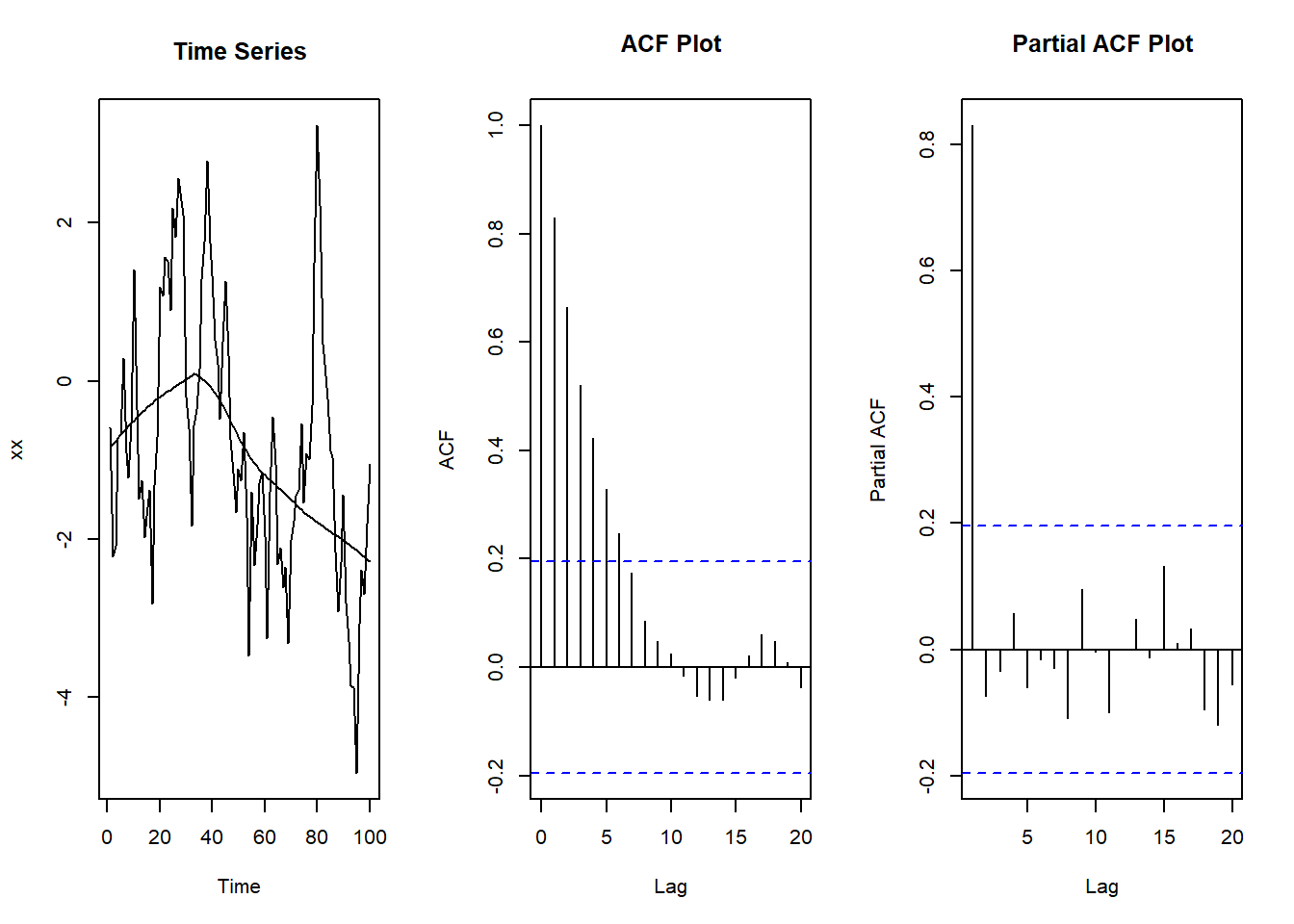
The arima.sim function generates a time series based on an autoregressive integrated moving average (ARIMA) model. The time series plot indicates the data tend to remain high or low, which is the positive autocorrelation. Because this is an AR(1) time series, its autocorrelation function decays and its partial autocorrelation function drops off after lag 1.

Using the Kendall and zyp libraries, we can run the Mann-Kendall test and pre-whitened Mann-Kendall test, respectively, on the time series data:

library(Kendall)
MannKendall(xx)

## tau = -0.27, 2-sided pvalue =7.0147e-05

library(zyp)
zyp.trend.vector(
  xx, method = 'yuepilon',
  conf.intervals = TRUE,
  preserve.range.for.sig.test = TRUE
)

##      lbound       trend      trendp      ubound         tau         sig 
## -0.03438398 -0.02264216 -2.26421647 -0.01201662 -0.10781281  0.11454801 
##       nruns     autocor  valid_frac      linear   intercept 
##  1.00000000  0.79744803  1.00000000 -0.02188805  0.17044683

The p-value of the Mann-Kendall test is <0.001, indicating a statistically significant trend. After removal of the positive serial correlation component from the time series by pre-whitening, the corrected p-value is 0.115. The data were generated to have no trend, so the apparent trend based on the Mann-Kendall test is due to the autocorrelation. No trend in the data was correctly identified by the pre-whitened test.

A closely related problem is the case where seasonality exists in the data. By dividing the observations into separate classes according to the season and then performing the Mann-Kendall trend test on the sum of the statistics from each season, the effect of seasonality can be eliminated. This modification is called the Seasonal Kendall test (Hirsch et al. 1982; Hirsch and Slack 1984). Although the seasonal test eliminates the effect of seasonal dependence, it does not account for correlation in the series within the season (Hirsch and Slack 1984).

Theil-Sen Line

The Theil-Sen method is used in conjunction with the Mann-Kendall test to determine a slope, or rate of change, of the trending data (Helsel 2012). Although nonparametric, the Theil-Sen method does not use data ranks but rather the concentrations themselves. The essential idea is that if a simple slope estimate is computed for every pair of distinct measurements in the sample (known as the set of pairwise slopes), the average of this series of slope values should approximate the true slope. The Theil-Sen method is nonparametric because instead of taking an arithmetic average of the pairwise slopes, the median slope value is determined. Consequently, the Theil-Sen line estimates the change in median concentration over time.

The Theil-Sen method handles nondetects in the same manner as the Mann-Kendall test; it assigns each nondetect a common value less than any detected measurement (USEPA 2009). Unlike the Mann-Kendall test, however, the actual concentration values are important in computing the slope estimate in the Theil-Sen procedure. Larger proportions of nondetect data make computation of the Theil-Sen trend line uncertain and the approach is not appropriate when more than 50 percent of the measurements are nondetects (ITRC 2013).

An alternative to the Thiel-Sen line is the Akritas-Theil-Sen (ATS) trend line with Turnbull estimate of intercept (Helsel 2012). The ATS procedure iteratively solves for a slope while the Theil-Sen slope is directly computed because nondetects are assigned a proxy value. After computing the slope, there are several ways to compute an intercept. The approach used by USEPA (2009) fits the line through the point (median of x, median of y) and then solves for the intercept. An alternative approach is to set the intercept as the median residual of all y values minus the slope*x (referred to as the Turnbull estimate).

Let’s compare the two estimates using a dataset comprised of zinc concentrations measured quarterly in a single groundwater well between September 2013 and October 2017.

# Load libraries
library(ggplot2)
library(scales)

# Read data in comma-delimited file
dat <- read.csv('data/zinc.csv', header = T)
dat$LOGDATE <- as.POSIXct(dat$LOGDATE, format = '%m/%d/%Y')

str(dat)

## 'data.frame':	17 obs. of  7 variables:
##  $ LOCID   : chr  "MW-2" "MW-2" "MW-2" "MW-2" ...
##  $ LOGDATE : POSIXct, format: "2013-09-13" "2013-12-15" ...
##  $ PARAM   : chr  "Zinc" "Zinc" "Zinc" "Zinc" ...
##  $ DETECTED: chr  "Y" "Y" "Y" "Y" ...
##  $ RESULT  : num  21 29 20 22 10 20 14 10 5.1 5 ...
##  $ MDL     : int  10 10 10 10 10 10 10 10 5 5 ...
##  $ UNITS   : chr  "ug/L" "ug/L" "ug/L" "ug/L" ...

The data contain 17 observations and 7 variables. The variables include well id, sample date, parameter name, a detected flag, measurement result, method detection limit (MDL), and units of measurement.

Prior to the analyses, we need to assigned some new variables to the dataset.

# Assign the MDL to nondetects
minval <- min(dat[dat$DETECTED == 'Y',]$RESULT)
dat <- within(dat, {
    RESULT = ifelse(DETECTED == 'Y', RESULT, MDL)
})

# Assign one-half the MDL to nondetects
minval <- min(dat[dat$DETECTED == 'Y',]$RESULT)
dat <- within(dat, {
    RESULT2 = ifelse(DETECTED == 'Y', RESULT, 0.5*MDL)
})

# Assign a value less than the lowest detected value to nondetects
minval <- min(dat[dat$DETECTED == 'Y',]$RESULT)
dat <- within(dat, {
    RESULT3 = ifelse(DETECTED == 'Y', RESULT, 0.5*minval)
})

# Add censored column
dat$CENSORED <- ifelse(dat$DETECTED == 'N', TRUE, FALSE)

# Add decimal date to data
d <- as.POSIXct('1/1/1970', format = "%m/%d/%Y")
yr <- as.numeric(
  round(1970 + difftime(dat$LOGDATE, d, units = 'days')/365.25, 4)
)
dat <- cbind(dat, DATE = yr)

Let’s compute the Theil-Sen regression estimator.

# Function to compute Theil-Sen regression estimator
theilsen <- function(x,y){ 
  ord <- order(x) 
  xs <- x[ord] 
  ys <- y[ord] 
  vec1 <- outer(ys, ys, "-") 
  vec2 <- outer(xs, xs, "-") 
  v1 <- vec1[vec2 > 0] 
  v2 <- vec2[vec2 > 0] 
  slope <- median(v1/v2)
  coef <- median(y) - slope * median(x)
  c(coef, slope) 
}

# Compute Theil-Sen regression coefficients   
sen <- with(dat, theilsen(DATE, RESULT3))
sen

## [1] 10640.224685    -5.275747

Let’s compute the ATS trend line with Turnbull estimate of intercept.

# Compute Akritas-Theil-Sen line with Turnbull estimate of intercept
library(NADA)
datken <- with(dat, cenken(RESULT, CENSORED, DATE))
datken

## $slope
## [1] -6.553709
## 
## $intercept
## [1] 13220.92
## 
## $tau
## [1] -0.5882353
## 
## $p
## [1] 0.0008732508
## 
## attr(,"class")
## [1] "cenken"

Now that we have regressed the data, let’s plot the data showing both trend lines.

# Create time-series plot
p <- ggplot(data = dat, aes(x = DATE, y = RESULT2, shape = DETECTED)) +
   geom_point(color = 'black', size = 3, stroke = 1.1) +
   scale_x_continuous(limits = c(2013, 2018),
                      breaks = seq(2013, 2018, by = 1)) +
   scale_y_continuous(limits = c(0, 1.1*max(dat$RESULT2)),
                      labels = function(x) format(x, big.mark = ",",
                                                  scientific = FALSE)) +
   labs(title = 'Nonparametric Trend Line Comparison',
        subtitle = 'Theil-Sen = blue line\nAkritas-Theil-Sen = red line',
        caption = 'Open symbols represent nondetects plotted at one-half the MDL.',
        x = 'Year',
        y = paste0("Result (", "\u03bc", "g/L)")) +
   scale_shape_manual(values = c('N' = 1,
                                 'Y' = 16),
                      guide = "none") +
   theme_bw() +
   theme(plot.title = element_text(margin = margin(b = 2), size = 14, hjust = 0.0,
                                   color = 'black', face = quote(bold)),
         plot.subtitle = element_text(margin = margin(b = 4), size = 11, hjust = 0.0,
                                      color = 'black', face = quote(italic)),
         plot.caption = element_text(size = 9),
         axis.title.y = element_text(size = 13, color = 'black'),
         axis.title.x = element_text(size = 13, color = 'black'),
         axis.text.x = element_text(size = 11, color = 'black'),
         axis.text.y = element_text(size = 11, color = 'black'))

# Add Theil-Sen line
p <- p +
  geom_segment(x = min(dat$DATE),
               y = min(dat$DATE)*sen[2] + sen[1],
               xend = max(dat$DATE),
               yend = max(dat$DATE)*sen[2] + sen[1],
               color = 'blue', size = 1)

# Add Akritas-Theil-Sen line
p <- p +
  geom_segment(x = min(dat$DATE),
               y = min(dat$DATE)*datken$slope + datken$intercept,
               xend = max(dat$DATE),
               yend = max(dat$DATE)*datken$slope + datken$intercept,
                color = 'red', size = 1)
p

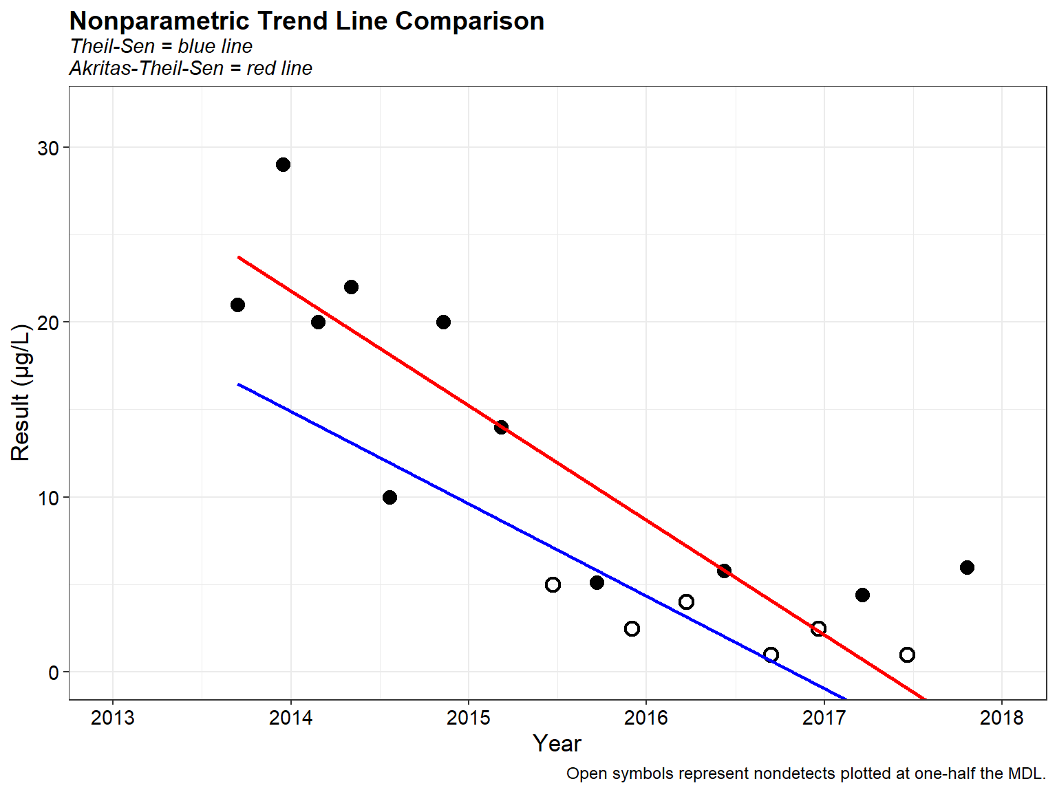
The two trend lines and especially the intercepts are different. For the ATS line, about half the data are above the line and half below the line. This is not the case with the Theil-Sen line where most of the data are above the line. The ATS trend line is preferred because the Theil-Sen method of using the median of x and y individually is not necessarily a good center point of the data. In the presence of nondetects, the ATS line provides a better estimate because the Theil-Sen line cannot be computed without substituting some unknown value for nondetects.

Uncertainty

To understand uncertainty associated with the trend line, confidence bands around the trend line can be constructed using bootstrapping. In this method, the Theil-Sen trend is first computed using the sample data. Then a large number of bootstrap resamples are drawn from the original sample, and an alternate Theil-Sen trend is conducted on each bootstrap sample. Variability in these alternate trend estimates is used to construct a confidence band around the original trend. Because nondetect values are known to be within an interval between zero and the detection or reporting limit, representing these values by an interval, such as with a line segment, provides a visual picture of what is known about the data. These censored scatterplots can be used to more clearly illustrate the interval-censoring of the data. An example of a censored Theil-Sen trend plot with bootstrapped confidence bands is shown below.

References

Gilbert, R.O. 1987. Statistical Methods for Environmental Pollution Monitoring. Wiley, New York.

Hamed, K. H. and R.A. Ramachandra. 1998. A modified Mann-Kendall trend test for autocorrelated data. Journal of Hydrology 204, 182-196

Helsel, D.R. 2012. Statistics for Censored Environmental Data Using Minitab and R, 2nd Edition. John Wiley and Sons, New Jersey.

Hirsch, R.M., J.R., Slack, and R.A. Smith. 1982. Techniques of trend analysis for monthly water quality data. Water Resources Research 18, 107-121.

Hirsch, R. M. and J.R. Slack. 1984. A nonparametric trend test for seasonal data with serial dependence. Water Resources Research 20, 727-732.

Interstate Technology & Regulatory Council (ITRC). 2013. Groundwater Statistics and Monitoring Compliance: Statistical Tools for the Project Life Cycle. GSMC-1. December.

Kendall, M. G. 1975. Rank Correlation Methods. Charles Griffin, London.

Mann, H. B. 1945. Non-parametric tests against trend. Econometrica 13, 245-259.

U.S. Environmental Protection Agency (USEPA). 2009. Statistical Analysis of Groundwater Monitoring Data at RCRA Facilities-Unified Guidance. EPA 530/R-09-007. Office of Research and Development. March.

Yue, S. and C.Y. Wang. 2002. Applicability of prewhitening to eliminate the influence of serial correlation on the Mann-Kendall test. Water Resources Research 38, 4-1-4-7.

Yue, S. and C.Y. Wang. 2004. The Mann-Kendall test modified by effective sample size to detect trend in serially correlated hydrological series. Water Resources Management 18, 201-218.