Outlier Detection Using Machine Learning
By Charles Holbert
September 9, 2019
Introduction
A difficult problem in data analysis is dealing with outliers in a set of data. An outlier is an observation with a value that does not appear to belong with the rest of the values in the dataset. There is no precise way to define and identify outliers in general because of the specifics of each dataset. Instead, the data analyst, must interpret the raw observations and decide whether a value is an outlier or not. Statistical methods are available to identify observations that appear to be rare or unlikely given the available data. These methods include both graphical representations of the data and formal statistical tests. When there are multiple outliers in a dataset, identification becames more complicated. For instance, one outlier may mask another outlier in a single outlier test. Thus, it is important to inspect the data graphically for the presence of outliers prior to formal testing.
Outliers may be univariate or multivariate. Multivariate outliers are observations that are inconsistent with the correlational structure of the dataset. Thus, while univariate outlier detection is performed independently on each variable, multivariate methods investigate the relationship of several variables. A multivariate outlier is an observation with characteristics different from the multivariate distribution of the majority of the observations. Detection of multivariate outliers is a much more difficult task than detecting univariate outliers because there are several directions in which a point can be outlying.
It’s important to note that statistical tests are used to identify outliers, not to reject them from the dataset. Generally, an observation should not be removed from the dataset unless an investigation finds a probable cause to justify its removal. Many statistical tests for outlier detection determine the likelihood of an observation being an outlier if the data, excluding the outlier, follow a normal distribution. Most data from the natural world follow skewed, not normal, distributions. Thus, a test that relies on an assumption of a normal distribution may identify a relatively large number of statistical outliers caused by common skewness, not necessarily erroneous or anomalous observations.
In this post, we will investigate three methods for multivariate outlier detection: Mahalanobis distance (a multivariate extension to standard univariate tests) and two machine learning (clustering) techniques.
Parameters
Several libraries, functions, and parameters are required to perform the outlier analyses.
# Load libraries
library(knitr)
library(ggplot2)
library(data.table)
library(GGally)
library(robustbase)
library(dbscan)
library(mclust)

# Load mvOutlier function
source('./functions/mvOutlier.R')
Data
For this example, let’s use one of R’s sample datasets, mtcars. The mtcars dataset was extracted from the 1974 Motor Trend US magazine, and comprises fuel consumption and 10 aspects of automobile design and performance for the 1973 to 1974 models of 32 automobiles (source: https://stat.ethz.ch/R-manual/R-devel/library/datasets/html/mtcars.html). Let’s load the data and then inspect the general structure.
# Load data
data(mtcars)
str(mtcars)
## 'data.frame':	32 obs. of  11 variables:
##  $ mpg : num  21 21 22.8 21.4 18.7 18.1 14.3 24.4 22.8 19.2 ...
##  $ cyl : num  6 6 4 6 8 6 8 4 4 6 ...
##  $ disp: num  160 160 108 258 360 ...
##  $ hp  : num  110 110 93 110 175 105 245 62 95 123 ...
##  $ drat: num  3.9 3.9 3.85 3.08 3.15 2.76 3.21 3.69 3.92 3.92 ...
##  $ wt  : num  2.62 2.88 2.32 3.21 3.44 ...
##  $ qsec: num  16.5 17 18.6 19.4 17 ...
##  $ vs  : num  0 0 1 1 0 1 0 1 1 1 ...
##  $ am  : num  1 1 1 0 0 0 0 0 0 0 ...
##  $ gear: num  4 4 4 3 3 3 3 4 4 4 ...
##  $ carb: num  4 4 1 1 2 1 4 2 2 4 ...
Now, lets’ inspect the entire dataset.
# Inspect the data
kable(mtcars, caption = "mtcars Data")
Table: Table 1: mtcars Data
| mpg | cyl | disp | hp | drat | wt | qsec | vs | am | gear | carb | |
|---|---|---|---|---|---|---|---|---|---|---|---|
| Mazda RX4 | 21.0 | 6 | 160.0 | 110 | 3.90 | 2.620 | 16.46 | 0 | 1 | 4 | 4 |
| Mazda RX4 Wag | 21.0 | 6 | 160.0 | 110 | 3.90 | 2.875 | 17.02 | 0 | 1 | 4 | 4 |
| Datsun 710 | 22.8 | 4 | 108.0 | 93 | 3.85 | 2.320 | 18.61 | 1 | 1 | 4 | 1 |
| Hornet 4 Drive | 21.4 | 6 | 258.0 | 110 | 3.08 | 3.215 | 19.44 | 1 | 0 | 3 | 1 |
| Hornet Sportabout | 18.7 | 8 | 360.0 | 175 | 3.15 | 3.440 | 17.02 | 0 | 0 | 3 | 2 |
| Valiant | 18.1 | 6 | 225.0 | 105 | 2.76 | 3.460 | 20.22 | 1 | 0 | 3 | 1 |
| Duster 360 | 14.3 | 8 | 360.0 | 245 | 3.21 | 3.570 | 15.84 | 0 | 0 | 3 | 4 |
| Merc 240D | 24.4 | 4 | 146.7 | 62 | 3.69 | 3.190 | 20.00 | 1 | 0 | 4 | 2 |
| Merc 230 | 22.8 | 4 | 140.8 | 95 | 3.92 | 3.150 | 22.90 | 1 | 0 | 4 | 2 |
| Merc 280 | 19.2 | 6 | 167.6 | 123 | 3.92 | 3.440 | 18.30 | 1 | 0 | 4 | 4 |
| Merc 280C | 17.8 | 6 | 167.6 | 123 | 3.92 | 3.440 | 18.90 | 1 | 0 | 4 | 4 |
| Merc 450SE | 16.4 | 8 | 275.8 | 180 | 3.07 | 4.070 | 17.40 | 0 | 0 | 3 | 3 |
| Merc 450SL | 17.3 | 8 | 275.8 | 180 | 3.07 | 3.730 | 17.60 | 0 | 0 | 3 | 3 |
| Merc 450SLC | 15.2 | 8 | 275.8 | 180 | 3.07 | 3.780 | 18.00 | 0 | 0 | 3 | 3 |
| Cadillac Fleetwood | 10.4 | 8 | 472.0 | 205 | 2.93 | 5.250 | 17.98 | 0 | 0 | 3 | 4 |
| Lincoln Continental | 10.4 | 8 | 460.0 | 215 | 3.00 | 5.424 | 17.82 | 0 | 0 | 3 | 4 |
| Chrysler Imperial | 14.7 | 8 | 440.0 | 230 | 3.23 | 5.345 | 17.42 | 0 | 0 | 3 | 4 |
| Fiat 128 | 32.4 | 4 | 78.7 | 66 | 4.08 | 2.200 | 19.47 | 1 | 1 | 4 | 1 |
| Honda Civic | 30.4 | 4 | 75.7 | 52 | 4.93 | 1.615 | 18.52 | 1 | 1 | 4 | 2 |
| Toyota Corolla | 33.9 | 4 | 71.1 | 65 | 4.22 | 1.835 | 19.90 | 1 | 1 | 4 | 1 |
| Toyota Corona | 21.5 | 4 | 120.1 | 97 | 3.70 | 2.465 | 20.01 | 1 | 0 | 3 | 1 |
| Dodge Challenger | 15.5 | 8 | 318.0 | 150 | 2.76 | 3.520 | 16.87 | 0 | 0 | 3 | 2 |
| AMC Javelin | 15.2 | 8 | 304.0 | 150 | 3.15 | 3.435 | 17.30 | 0 | 0 | 3 | 2 |
| Camaro Z28 | 13.3 | 8 | 350.0 | 245 | 3.73 | 3.840 | 15.41 | 0 | 0 | 3 | 4 |
| Pontiac Firebird | 19.2 | 8 | 400.0 | 175 | 3.08 | 3.845 | 17.05 | 0 | 0 | 3 | 2 |
| Fiat X1-9 | 27.3 | 4 | 79.0 | 66 | 4.08 | 1.935 | 18.90 | 1 | 1 | 4 | 1 |
| Porsche 914-2 | 26.0 | 4 | 120.3 | 91 | 4.43 | 2.140 | 16.70 | 0 | 1 | 5 | 2 |
| Lotus Europa | 30.4 | 4 | 95.1 | 113 | 3.77 | 1.513 | 16.90 | 1 | 1 | 5 | 2 |
| Ford Pantera L | 15.8 | 8 | 351.0 | 264 | 4.22 | 3.170 | 14.50 | 0 | 1 | 5 | 4 |
| Ferrari Dino | 19.7 | 6 | 145.0 | 175 | 3.62 | 2.770 | 15.50 | 0 | 1 | 5 | 6 |
| Maserati Bora | 15.0 | 8 | 301.0 | 335 | 3.54 | 3.570 | 14.60 | 0 | 1 | 5 | 8 |
| Volvo 142E | 21.4 | 4 | 121.0 | 109 | 4.11 | 2.780 | 18.60 | 1 | 1 | 4 | 2 |
We see that the mtcars dataset consists of a data frame with 32 observations on 11 (numeric) variables given as follows:
[, 1] mpg Miles/(US) gallon
[, 2] cyl Number of cylinders
[, 3] disp Displacement (cu.in.)
[, 4] hp Gross horsepower
[, 5] drat Rear axle ratio
[, 6] wt Weight (1000 lbs)
[, 7] qsec 1/4 mile time
[, 8] vs Engine (0 = V-shaped, 1 = straight)
[, 9] am Transmission (0 = automatic, 1 = manual)
[,10] gear Number of forward gears
[,11] carb Number of carburetors\
Let’s visually inspect a few of the variables to see if the data contain any obvious outliers.
# Create pairs plot using GGally
ggpairs(mtcars[, c("mpg", "cyl", "hp", "qsec")])

The hp and qsec variables may contain a few outliers, but it’s difficult to ascertain by inspecting these plots. To assist with visualization, let’s use principal component analysis (PCA) to create a simple two-dimensional mapping of the data.
Principal Component Analysis
PCA is a useful statistical tool for analyzing multivariate data. PCA uses spectral (eigenvalue) decomposition to transform a number of correlated variables into a smaller number of uncorrelated variables, called principal components (PCs), with a minimum loss of information (Joliffe 1986). These new variables are linear combinations of the original variables.\
PCA requires that the input variables have similar scales of measurement and when comparing variables that have different units of measure and different variances, the data need to be standardized. Let’s standardize the mtcars data by mean-centering and scaling to unit variance prior to conducting PCA.
distance_matrix <- as.matrix(dist(scale(mtcars)))
pca <- prcomp(distance_matrix)

mtcars.dt <- data.table(pca$x[, 1:2])
mtcars.dt[, CarNames := rownames(mtcars)]

ggplot(mtcars.dt, aes(x = PC1, y = PC2)) +
  geom_point(size = 10, color = "steelblue", alpha = 0.3) +
  geom_text(aes(label = CarNames), check_overlap = TRUE) +
  theme_minimal()
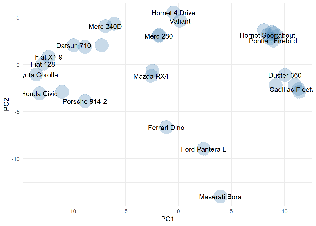
This two-dimensional visualization is easier to view and suggests the presence of some possible outliers (Ferrari Dino, Ford Panterra, and Maserati Bora). Now, let’s explore outlier detection using cluster analysis.
Cluster Analysis
Cluster analysis involves the classification of data objects into similarity groups (clusters) according to a defined distance measure. In the process, data in the same group have maximum similarity, while data in different groups have minimum similarity. Clustering is extensively used in fields such as machine learning, data mining, pattern recognition, geological exploration, image analysis, genomics, and biology.
The traditional clustering methods, such as hierarchical clustering and k-means clustering, are based on heuristic algorithms. Most heuristic clustering algorithms suffer from the problem of being sensitive to the initialization so different runs will often yield different results. An alternative approach is model-based clustering, which consider the data as coming from a distribution that is mixture of two or more clusters (Fraley and Raftery 2002). Each component (i.e., cluster) is modeled by the normal or Gaussian distribution where the model parameters are estimated using the Expectation-Maximization (EM) algorithm initialized by hierarchical model-based clustering. Unlike heuristic-based clustering, the model-based clustering approach uses a soft assignment, where each data point has a probability of belonging to each cluster.
Mahalanobis Distance
Although not strictly a machine learning method, Mahalanobis distance is an extension of the univariate z-score that accounts for the correlation structure between features of a dataset. Mahalanobis distance is an effective multivariate metric that measures the distance between a point and a distribution. It is effectively a multivariate equivalent of the Euclidean distance. Because Mahalanobis distance uses the multivariate sample mean and covariance matrix, it is useful for identifying outliers when data are multivariate normal.
Mahalanobis distance is primarily used in classification and clustering problems where there is a need to establish correlation between different groups/clusters of data. Another application of Mahalanobis distance is discriminant analysis and pattern analysis, which are based on classification. It has also found relevance in PCA for detecting outliers in multidimensional data. Under the null hypothesis that all samples arise from the same multivariate normal distribution, the distance from the center of a d-dimensional PC space follows a chi-squared distribution with d degrees of freedom. The p-values associated with the Mahalanobis distances can then be calcuated for each observation.
Let’s compute the Mahalanobis distance using our mtcars dataset and use the results to compare to the machine learning (clustering) methods for outlier detection.
set.seed(4351)
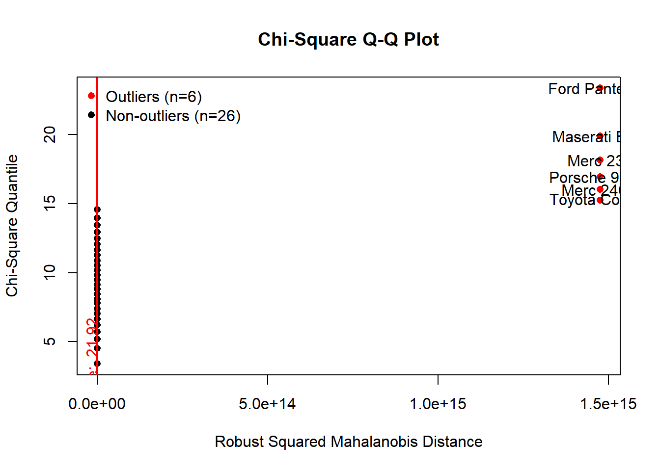
results <- mvOutlier(scale(mtcars), qqplot = TRUE, method = "quan")
results <- data.table(
  CarNames = rownames(results$outlier),
  MDOutlier = results$outlier$Outlier
)
mtcars.dt <- merge(mtcars.dt, results, by = "CarNames")

ggplot(mtcars.dt, aes(x = PC1, y = PC2)) +
  geom_point(aes(color = MDOutlier), size = 10, alpha = 0.3) +
  geom_text(aes(label = CarNames), check_overlap = TRUE) +
  scale_color_manual(name = "MD Outlier", values = c("steelblue", "red")) +
  theme_minimal()
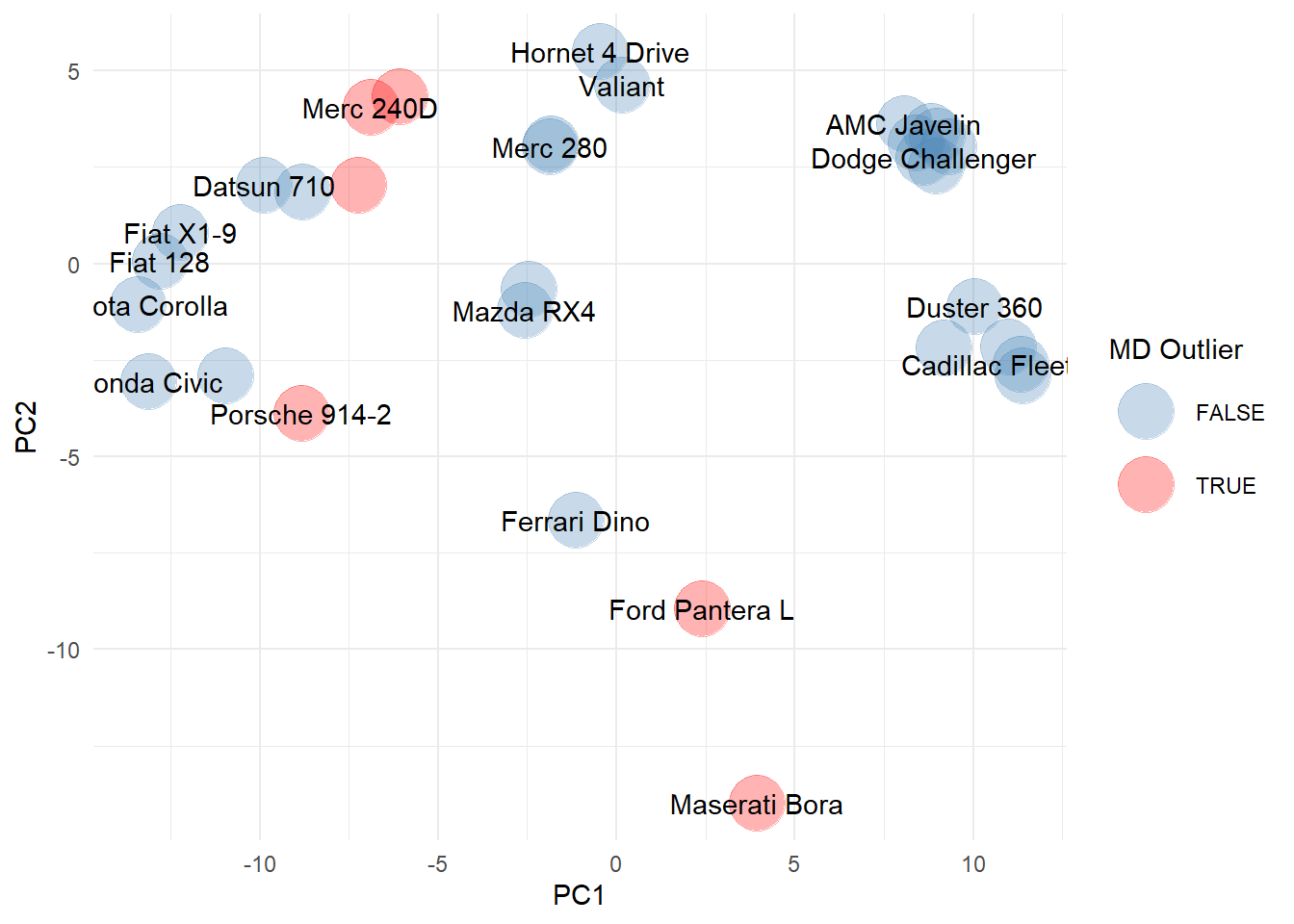
The Mahalanobis distance indicates the Ford Panetra and Maserati Bora may be outliers in the dataset. It also highlights other cars (note some labels are missing due to overlap), including the Merc 280, Merc 280D, Toyota Corona, and Porsche 914. These cars are an interesting mix of super cars (e.g., Maserati and Porsche) and older cars (e.g., Toyota Corona and Mercs), that clearly bear little resemblance to the remaining cars in the dataset.
Density-Based Spatial Clustering and Application with Noise
The Density-Based Spatial Clustering and Application with Noise (DBSCAN) algorithm introducted by Ester et al. (1996) is designed to discover clusters of arbitrary shape in a dataset containing noise and outliers. Unlike K-means clustering, DBSCAN does not require the user to specify the number of clusters to be generated. Two important parameters are required for DBSCAN. These include the parameter eps, which defines the radius of the neighborhood around a point, and the parameter MinPts, which is the minimum number of neighbors within the specified radius. Any point within eps around one of its members (the seed) is considered a cluster member (recursively). Some points may not belong to any clusters and are treated as outliers or noise. If eps is too small, sparser clusters will be defined as noise and if eps is too large, denser clusters may be merged together.
Let’s run the DBSCAN algorithm on our data.
db <- dbscan(scale(mtcars), eps = 2, minPts = 3)$cluster

results <- data.table(
  CarNames = rownames(mtcars),
  DClusters = db
)
mtcars.dt <- merge(mtcars.dt, results, by = "CarNames")

ggplot(mtcars.dt, aes(x = PC1, y = PC2)) +
  geom_point(aes(color = factor(DClusters)), size = 10, alpha = 0.3) +
  geom_text(aes(label = CarNames), check_overlap = TRUE) +
  scale_color_hue(name = "DCluster", l = 40) +
  theme_minimal()
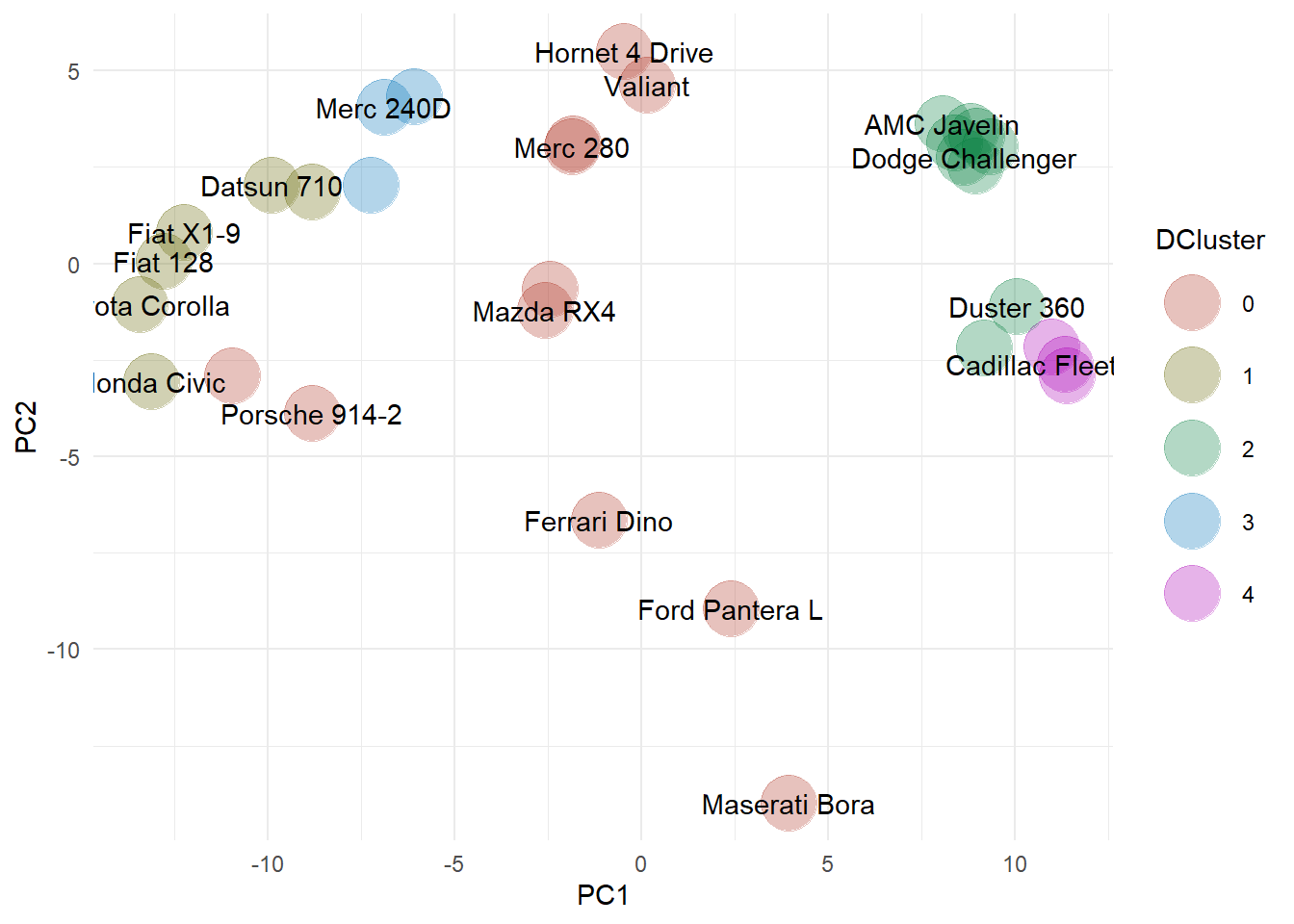
The outliers are assigned cluster 0, shown as the orange symbols in the PCA plot. There is a clear band of outliers through the center, with some overlap with the results from the Mahalanobis distances. However, there are clearly some differences between the two methods, mainly associated with the differing assumptions between the two methods. For example, DBSCAN identifies the Mazdas, the Hornet, the Lotus, and the Valiant as outliers. Remember that this is a density-based algorithm, so given the neighborhood and density that we defined, there are not enough similar cars in this dataset to say that these cars are “representative” or “normal”. This makes sense if you think of density as a kind of popularity measure. Interesting are the clusters that DBSCAN found. There is a small car cluster (1), a Mercedes cluster (3) and two muscle car clusters (2 and 4).
Expectation Maximization
The R package mclust is a popular package which allows modelling of data as a Gaussian finite mixture with different covariance structures and different numbers of mixture components, for a variety of purposes of analysis (Scrucca et al. 2016). The EM algorithm is used for maximum likelihood estimation where initialization is performed using the partitions obtained from agglomerative hierarchical clustering. It is an unsupervised clustering algorithm that tries to find similar subspaces based on their orientation and variance. The best model is selected using the Bayesian Information Criterion or BIC. A large BIC score indicates strong evidence for the corresponding model.
Let’s run the EM clustering method on our data.
cars_em <- Mclust(scale(mtcars), G = 4)

results <- data.table(
  CarNames = names(cars_em$classification),
  EMClusters = cars_em$classification
)
mtcars.dt <- merge(mtcars.dt, results, by = "CarNames")

ggplot(mtcars.dt, aes(x = PC1, y = PC2)) +
  geom_point(aes(color = factor(EMClusters)), size = 10, alpha = 0.3) +
  geom_text(aes(label = CarNames), check_overlap = TRUE) +
  scale_color_hue(name = "EMCluster", l = 40) +
  theme_minimal()
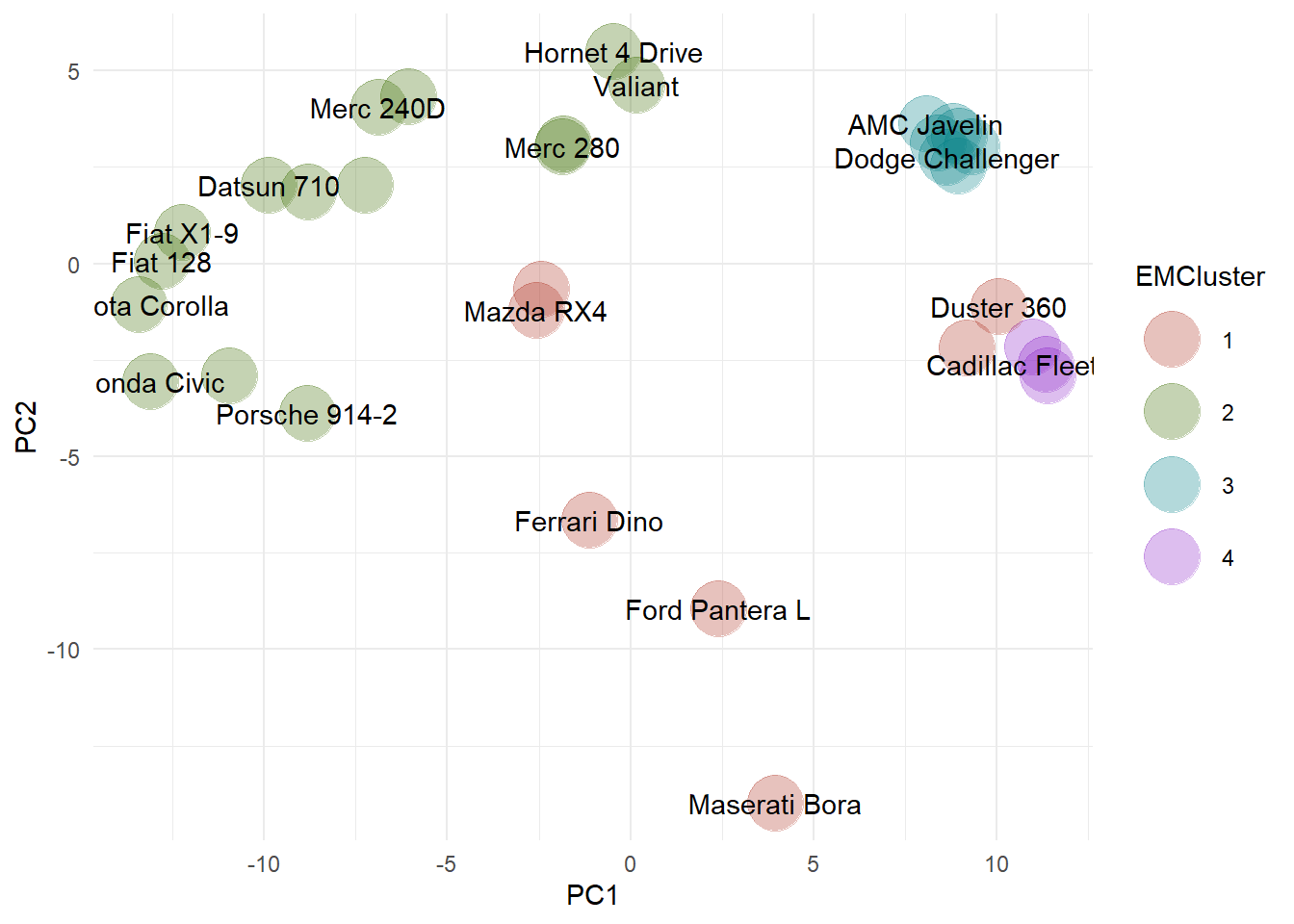
The outliers are assigned cluster 1, shown as the orange symbols in the PCA plot. Outliers identified using the EM method include the Ferrari, the Ford Pantera, and the Maserati.. Similar to the results obtained using the DBSCAN algorithm, the two Mazda RX4s are identified as outliers.
Let’s inspect the final results of the outlier identification using Mahalanobis distance and the two clusting methods.
kable(mtcars.dt, digits = 2, align = c("l", rep("c", 5)),
      caption = "Final Results")
Table: Table 2: Final Results
| CarNames | PC1 | PC2 | MDOutlier | DClusters | EMClusters |
|---|---|---|---|---|---|
| AMC Javelin | 8.07 | 3.64 | FALSE | 2 | 3 |
| Cadillac Fleetwood | 11.34 | -2.60 | FALSE | 4 | 4 |
| Camaro Z28 | 9.17 | -2.19 | FALSE | 2 | 1 |
| Chrysler Imperial | 10.97 | -2.15 | FALSE | 4 | 4 |
| Datsun 710 | -9.88 | 2.04 | FALSE | 1 | 2 |
| Dodge Challenger | 8.62 | 2.76 | FALSE | 2 | 3 |
| Duster 360 | 10.04 | -1.10 | FALSE | 2 | 1 |
| Ferrari Dino | -1.13 | -6.64 | FALSE | 0 | 1 |
| Fiat 128 | -12.78 | 0.07 | FALSE | 1 | 2 |
| Fiat X1-9 | -12.23 | 0.81 | FALSE | 1 | 2 |
| Ford Pantera L | 2.39 | -8.95 | TRUE | 0 | 1 |
| Honda Civic | -13.12 | -3.05 | FALSE | 1 | 2 |
| Hornet 4 Drive | -0.47 | 5.50 | FALSE | 0 | 2 |
| Hornet Sportabout | 8.38 | 3.13 | FALSE | 2 | 3 |
| Lincoln Continental | 11.39 | -2.90 | FALSE | 4 | 4 |
| Lotus Europa | -10.96 | -2.92 | FALSE | 0 | 2 |
| Maserati Bora | 3.95 | -13.99 | TRUE | 0 | 1 |
| Mazda RX4 | -2.57 | -1.20 | FALSE | 0 | 1 |
| Mazda RX4 Wag | -2.45 | -0.66 | FALSE | 0 | 1 |
| Merc 230 | -7.24 | 2.03 | TRUE | 3 | 2 |
| Merc 240D | -6.88 | 4.06 | TRUE | 3 | 2 |
| Merc 280 | -1.86 | 3.04 | FALSE | 0 | 2 |
| Merc 280C | -1.83 | 3.10 | FALSE | 0 | 2 |
| Merc 450SE | 9.32 | 3.04 | FALSE | 2 | 3 |
| Merc 450SL | 8.81 | 3.44 | FALSE | 2 | 3 |
| Merc 450SLC | 8.97 | 3.30 | FALSE | 2 | 3 |
| Pontiac Firebird | 8.95 | 2.53 | FALSE | 2 | 3 |
| Porsche 914-2 | -8.82 | -3.89 | TRUE | 0 | 2 |
| Toyota Corolla | -13.43 | -1.07 | FALSE | 1 | 2 |
| Toyota Corona | -6.07 | 4.33 | TRUE | 3 | 2 |
| Valiant | 0.16 | 4.63 | FALSE | 0 | 2 |
| Volvo 142E | -8.81 | 1.85 | FALSE | 1 | 2 |
Conclusions
There is agreement between the three methods that the Ford Pantera and the Maserati are outliers in this dataset. Depending on which method you choose, there are other cars which might also be outliers. This is a typical problem with machine learning (and statistics in general), that your results are reliant on the methods used to conduct the analysis. When conducting these types of analyses, it’s important to understand the assumptions for each method and how the data fit within those assumptions. For this example, our dataset is relatively small (32 cars), which makes it difficult to select the best algorithm or result. With such a small dataset, it’s difficult to accurately estimate the variance in the data and thus, Mahalanobis distance and the EM method may contain higher uncertainty than the DBSCAN method that relies on fewer assumptions.
Declaring an observation as an outlier based on a single feature could lead to unrealistic conditions. Deleting outliers is a science decision. It may be reasonable to delete occasional wild values from a stable (e.g., electronic) process, but generally it is not reasonable to delete field data collected by a representative sampling method. Field data will contain values that are identified as outliers in comparison to a normal distribution because most data from the natural world follow skewed (not normal) distributions. A statistical test cannot tell you whether an observation is “bad” and should be removed. It only tells you whether the observation was likely to have come from a normal distribution, and data identified as outliers due to common skewness don’t necessarily indicate bad data.
References
Ester, M., H. Kriegel, J. Sander, and X. Xu. 1996. A Density-Based Algorithm for Discovering Clusters in Large Spatial Databases with Noise. Institute for Computer Science, University of Munich. Proceedings of 2nd International Conference on Knowledge Discovery and Data Mining (KDD-96).
Fraley, C. and A.E. Raftery. 2002. Model-Based Clustering, Discriminant Analysis, and Density Estimation. Journal of the American Statistical Association, 97 (458): 611?31.
Jolliffe, I.T. 1986. Principal Component Analysis. Springer-Verlag, New York, New York.
Scrucca L, M. Fop, T.B. Murphy, and A.E. Raftery. 2016. mclust 5: Clustering, Classification and Density Estimation Using Gaussian Finite Mixture Models. The R Journal, 8, 205?233. https://journal.r-project.org/archive/2016-1/scrucca-fop-murphy-etal.pdf.
- Posted on:
- September 9, 2019
- Length:
- 15 minute read, 3121 words
- See Also: