Introduction

Ordinary least squares (OLS) regression is optimal when all regression assumptions are valid. When some of these assumptions are invalid, least squares regression can perform poorly. Robust regression is an alternative to least squares regression when data contain outliers or influential observations. Outliers tend to pull the least squares fit too far in their direction by receiving much more “weight” than they deserve. Typically, you would expect that the weight attached to each observation would be on average 1/n in a data set with n observations. However, outliers may receive considerably more weight, leading to distorted estimates of the regression coefficients. If the outliers are not influential, the regression curve may be of the correct shape, but the estimate of the standard error will be skewed, and confidence bands will be overly wide.

OLS Regression

Let’s create a dataset x and y, where y is a linear function of x.

# Set seed
set.seed(123)

mydata <- within(data.frame(x = 1:10), y <- rnorm(x, mean = x))
fm.orig <- lm(y ~ x, data = mydata)
coef(summary(fm.orig))

##              Estimate Std. Error   t value     Pr(>|t|)
## (Intercept) 0.5254674  0.6672766 0.7874806 4.536973e-01
## x           0.9180288  0.1075414 8.5365180 2.728816e-05

Now, let’s insert an outlier and refit the model.

mydata$y[2] <- 20
fm.lm <- update(fm.orig)
coef(summary(fm.lm))

##              Estimate Std. Error   t value  Pr(>|t|)
## (Intercept) 6.6021932   3.708910 1.7800898 0.1129350
## x           0.1446273   0.597745 0.2419549 0.8149021

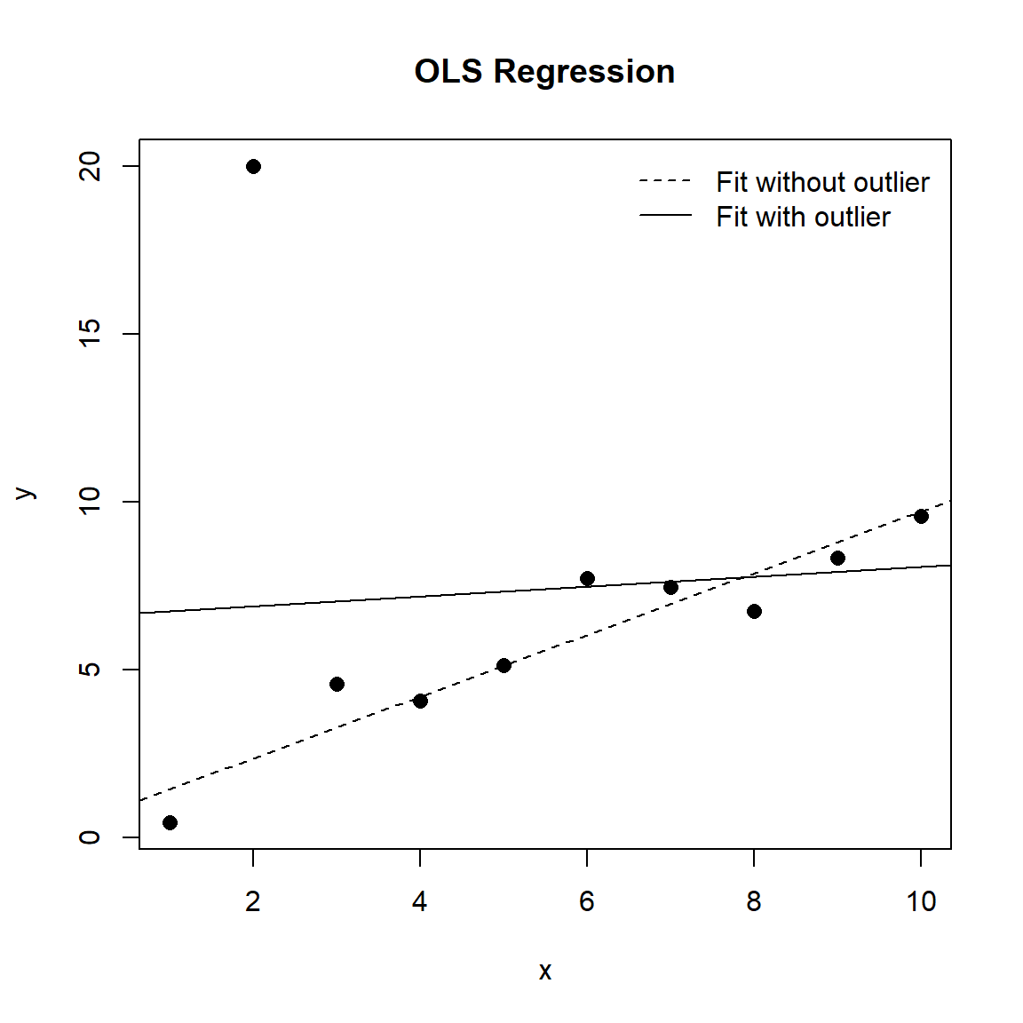
Comparing the coefficients of the two models, we see that the outlier has clearly biased both the slope and the intercept. Furthermore, the errors on both these parameters are greatly inflated. Let’s plot the two models to see how the regression lines fit the data.

#  Plot data and regression lines
plot(y ~ x, data = mydata, pch = 16, cex = 1.2, main = "OLS Regression")
abline(fm.orig, lty = "dashed")
abline(fm.lm)
legend(
  "topright", inset = 0.01, bty = "n",
  legend = c("Fit without outlier", "Fit with outlier"),
  lty = c("dashed", "solid")
)

The regression lines for the two models appear substantially different. Whereas the line for the model without the outlier fits the data quite well, the line with the outlier is heavily influenced by the single outlier.

Robust Regression

When we think of regression we usually think of estimating a mean of some variable conditional on the levels or values of independent variables. However, we don’t have to always estimate the conditional mean. We could estimate the median (or another quantile) and that’s where quantile regression (Koenker 2005) can be used. The math under the hood is a little different, but the interpretation is basically the same. In the end, we have regression coefficients that estimate an independent variable’s effect on a specified quantile of our dependent variable.

Using quantile regression, let’s model the median of y as a function of x, rather than modelling the mean of y as a function of x (as in the case of least squares regression).

# Robust regression using quantile regression
library(quantreg)
fm.rq <- rq(y ~ x, data = mydata)
coef(summary(fm.rq))

##             coefficients   lower bd  upper bd
## (Intercept)    0.7042374 -0.2682047 16.207800
## x              0.8850101 -0.4835863  1.170754

The “lower bd” and “upper bd” values are confidence intervals calculated using the rank method. Another common robust regression method falls into a class of estimators called M-estimators, introduced by Huber (1964). This method down-weights outliers according to how far they are from the best-fit line, and iteratively re-fits the model until convergence is achieved. Robust regression can be implemented using the rlm() function in the MASS package.

# Robust regression using MASS
library(MASS)
fm.rlm <- rlm(y ~ x, data = mydata)
coef(summary(fm.rlm))

##                 Value Std. Error  t value
## (Intercept) 1.7631738  0.9990055 1.764929
## x           0.7547735  0.1610043 4.687908

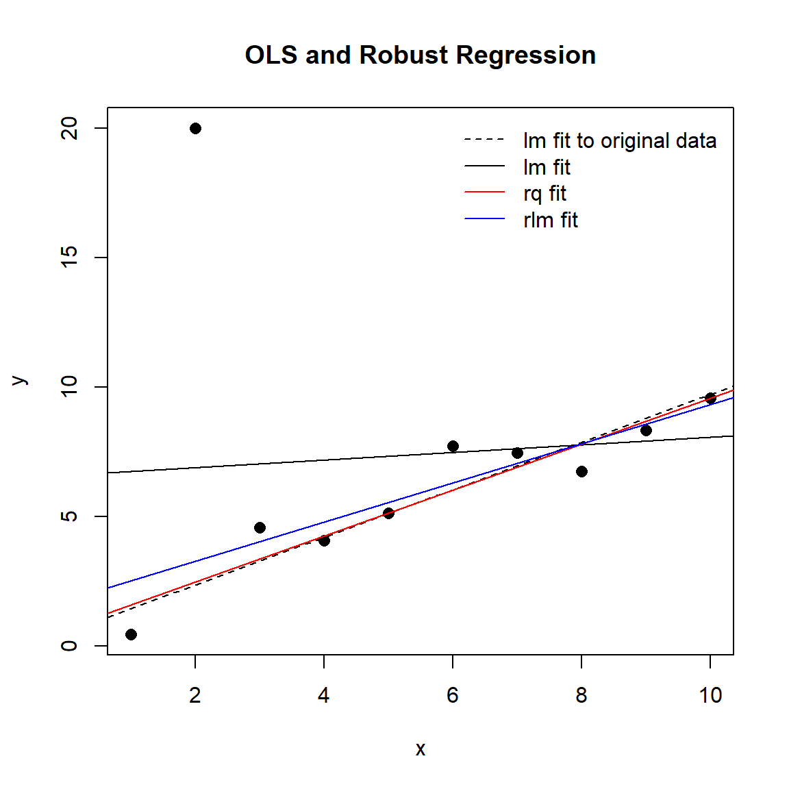
Now, let’s plot all the regression lines together for comparison.

plot(y ~ x, data = mydata, pch = 16, cex = 1.2, main = "OLS and Robust Regression")
abline(fm.orig, lty = "dashed")
abline(fm.lm)
abline(fm.rq, col = "red")
abline(fm.rlm, col = "blue")
legend(
  "topright", inset = 0.01, bty = "n",
  legend = c("lm fit to original data", "lm fit", "rq fit", "rlm fit"),
  lty = c(2, 1, 1, 1),
  col = c("black", "black", "red", "blue")
)

Both robust regression models succeed in resisting the influence of the outlier point and capturing the trend in the remaining data.

Conclusions

Robust regression can be used in any situation where OLS regression can be applied. It generally gives better accuracies over OLS when outliers are present because it uses a weighting mechanism to down-weight the influential observations. It is particularly resourceful when there are no compelling reasons to exclude outliers in your data because it is a compromise between excluding these points entirely from the analysis and treating all data equally in OLS regression. The idea of robust regression is to weigh the observations differently based on how well behaved these observations are. Roughly speaking, it is a form of weighted and re-weighted least squares regression.

Quantile regression is a highly versatile statistical modeling approach that does not assume a particular parametric distribution for the response, or a constant variance for the response, unlike least squares regression. Quantile regression yields valuable insights in applications such as risk management, where answers to important questions lie in modeling the tails of the conditional distribution. Although quantile regression is most often used to model specific conditional quantiles of the response, its full potential lies in modeling the entire conditional distribution. By comparison, standard least squares regression only models the conditional mean of the response.

For those interested in how quantile regression can be applied in the environmental sciences, see the publication by Cade and Noon (2003).

References

Cade, B. and B. Noon. 2003. A Gentle Introduction to Quantile Regression for Ecologists. Frontiers in Ecology and the Environment 1, 412-420.

Huber, P. J. 1964. Robust Estimation of a Location Parameter. Annals of Mathematical Statistics 35, 73-101.

Koenker, R. 2005. Quantile Regression (Econometric Society Monographs). Cambridge: Cambridge University Press.