Introduction

The United States Environmental Protection Agency (USEPA) guidance document Soil Screening Guidance: Technical Background Document, Second Edition (USEPA 1996) discusses sampling design and sample size calculations for studies to determine whether soil at a potentially contaminated site needs to be investigated for possible remedial action. Let’s use this document to compute the soil sample size necessary to achieve a specified power for a one-sample t-test, given the ratio of means, coefficient of variation, and significance level, assuming the data are lognormally distributed.

For this example, we will assume the investigative area is unlikely to be contaminated based on historical site use information or other site data that are reasonably complete and accurate. Because the investigative area is unlikely to be contaminated, concentrations of contaminants are expected to exhibit relatively low variability and the sampling design is based on a relatively small number of samples. If laboratory analytical results indicate greater variability associated with contamination patterns, additional samples may be required to determine with confidence whether the investigative area should be further evaluated.

Concentrations of contaminants detected in the surface soil samples will be evaulated using soil screening levels (SSLs). SSLs are concentrations of contaminants in soil that are designed to be protective of exposures in a residential setting. The USEPA used a default source area size of 0.5 acre to calculate the generic SSLs. However, generic SSLs based on a 0.5 acre source size are considered protective of larger sources as well because the EPA used an infinite source assumption (USEPA 1996).

The sampling data will be used to support a decision about whether the investigative area requires further study. Because of variability in contaminant concentrations within an investigative area, practical constraints on sample sizes, and sampling or measurement error, hypothesis tests will be used to control decision errors. When performing a hypothesis test, a presumed or baseline condition, referred to as the “null hypothesis” (Ho), is established. This baseline condition is presumed to be true unless the data conclusively demonstrate otherwise, which is called “rejecting the null hypothesis” in favor of an alternative hypothesis (Ha).

To complete the specification of limits on decision errors, Type I and Type II decision error probability limits must be defined in relation to the SSL. First a “gray region” is specified with respect to the mean contaminant concentration within the investigative area. The gray region represents the area where the consequences of decision errors are minor (and uncertainty in sampling data makes decisions too close to call). In other words, when the average of the data values is very close to the SSL, it would be too expensive to generate a data set of sufficient size and precision to resolve what the correct determination should be.

The USEPA (1996) established a default range for the width and location of the “gray region” that ranges from one-half the SSL (SSL/2) to two times the SSL (2*SSL). By specifying the upper edge of the gray region as twice the SSL, it is possible that exposure areas with mean values slightly higher than the SSL may be screened from further study. However, the USEPA (1996) believes that the exposure scenario and assumptions used to derive SSLs are sufficiently conservative to be protective in such cases.

Sample Size Requirement

Let ’theta’ denote the average concentration of the chemical of concern. The USEPA (1996, p.87) establishes the following goals for the decision rule:

          Pr[Decide Don’t Investigate | theta > 2 * SSL] = 0.05

          Pr[Decide to Investigate | theta <= (SSL/2)] = 0.20

where SSL denotes the pre-established soil screening level. These goals translate into a Type I error of 0.2 for the null hypothesis, and a power of 95% for the specific alternative hypothesis:

          H0: [theta / (SSL/2)] <= 1

          Ha: [theta / (SSL/2)] = 4

Most environmental data are right-skewed and can be represented by a lognormal distribution. Assuming the data are lognormally distributed, the sample size necessary to achieve a specified power for a one-sample t-test, given the ratio of means, and coefficient of variation (CV) can be calculated using the tTestLnormAltN() function in the EnvStats library (Millard, 2013) within the R language and environment for statistical computing (R Core Team, 2021). The USEPA (1996, p.88) recommends that a minimum default CV equal to 2.5 should be used when information is insufficient to estimate the CV. Under these conditions and assuming the above values for the Type I error and power, the minimum sample size:

# Load libraries
library(EnvStats)

N <- tTestLnormAltN(ratio.of.means = 4, cv = 2.5, alpha = 0.2,
                    alternative = "greater", approx = FALSE)
print(paste("Minimum sample size =", N), quote = F)

## [1] Minimum sample size = 7

Based on these calculations, at least 7 soil samples are required to satisfy the requirements for the Type I and Type II errors when the CV is 2.5.

The exact power associated with a sample size of 7 for this one-sample test is given by:

p <- tTestLnormAltPower(n.or.n1 = 7, ratio.of.means = 4,
                        cv = 2.5, alpha = 0.2,
                        alternative = "greater", approx = FALSE)
print(paste("Power =", round(p, 3)), quote = F)

## [1] Power = 0.954

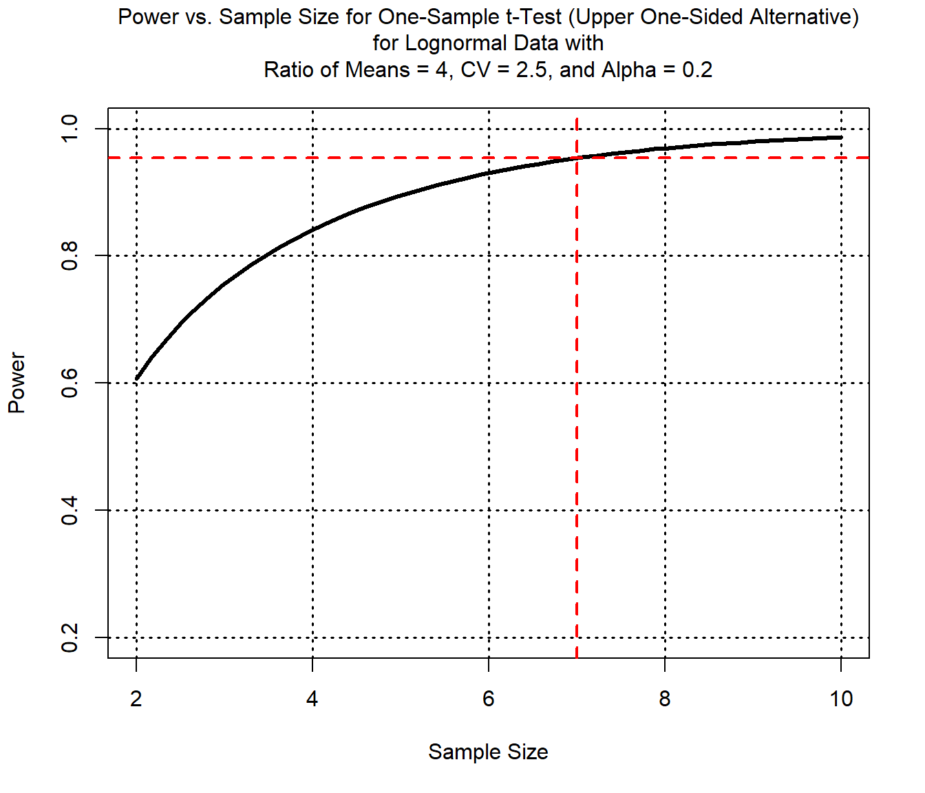
Assuming a lognormal distribution, a CV of 2.5, and the above values for the Type I error and power, a plot showing the power of a one-sample test versus sample size for a minimal detectable ratio of theta/(SSL/2) equal to 4 is given by:

plotTTestLnormAltDesign(x.var = "n", y.var = "power",
                        range.x.var = c(2, 10), ratio.of.means = 4,
                        cv = 2.5, alpha = 0.2,
                        alternative = "greater", approx = FALSE,
                        ylim = c(0.2, 1), xlab = "Sample Size")
grid(col = "black", lwd = 1.6)
abline(v = N, col = "red", lwd = 2, lty = 2)
abline(h = p, col = "red", lwd = 2, lty = 2)

References

Millard, S.P. 2013. EnvStats: An R Package for Environmental Statistics. Springer, NY.

R Core Team. 2021. R: A language and environment for statistical computing. R Foundation for Statistical Computing, Vienna, Austria. http://www.R-project.org.

U.S. Environmental Protection Agency (USEPA). 1996. Soil Screening Guidance: Technical Background Document, Second Edition. EPA/540/R-95/128. Office of Emergency and Remedial Response, U.S. Environmental Protection Agency, Washington, D.C., May, 1996.