Spatial Interpolation Using Integrated Nested Laplace Approximation
By Charles Holbert
January 19, 2021
Introduction
The performance of Bayesian inference using a stochastic partial differential equation (SPDE) approach with Integrated Nested Laplace Approximation (INLA) for predicting zinc concentrations in soil at unsampled locations is compared with those obtained using kriging. In the INLA-SPDE approach, a continuously indexed Gaussian random field is represented as a discretely indexed Gaussian Markov random field by means of a finite basis function defined on a triangulation of the region of study. The SPDE approach will be performed using the R-INLA package (Lindgren and Rue 2015).
Background
A point-referenced dataset is made up of data measured at known locations. These types of data are common in many areas, including mining, climate modeling, ecology, environmental science, and other fields. Point-referenced data are often obtained with the desire to elicit an underlying pattern thus, requiring development of a geospatial model of the data. Gaussian process modeling or a Gaussian stochastic process can be used to analyze these types of data. In geostatistics, Gaussian process modeling is referred to as kriging (Matheron 1963).
Kriging is a method of data interpolation based on predefined covariance models. The main idea of kriging is that near sample points should get more weight in the prediction at unsampled locations. Kriging relies on the knowledge of the spatial structure of the data, which is modeled using second-order properties (i.e., variogram or covariance) of the underlying random function Z(x). Kriging uses a weighted average of the observations \(Z(x_i)\) at the sample points \(x_i\) as the estimate.
There are several variants of kriging, including simple, ordinary, and universal kriging (Deutsch and Journel 1998). In ordinary kriging, the data are modeled as a Gaussian process with constant mean and a prescribed form of the stationary covariance function. The stationarity assumption reduces the number of hyperparameters and model complexity. In universal kriging, the assumption of constant mean is relaxed by modeling it as a polynomial, which increases the number of unknown parameters (Yang et al. 2018) .
Kriging can also be understood as a form of Bayesian inference (Williams 1998). Kriging starts with a prior distribution over functions. This prior takes the form of a Gaussian process, where the covariance between any two samples is the covariance function (or kernel) of the Gaussian process evaluated at the spatial location of two points. A set of values is then observed, each value associated with a spatial location. A new value can be predicted at any new spatial location, by combining the Gaussian prior with a Gaussian likelihood function for each of the observed values. The resulting posterior distribution is also Gaussian, with a mean and covariance that can be simply computed from the observed values, their variance, and the kernel matrix derived from the prior.
A commonly used covariance function is the Matérn covariance function (Cressie 2015). The covariance of two points which are a distance d apart is given by:
$$C_{v}(d) = \sigma^2\frac{2^{1-v}}{\Gamma(v)}(\sqrt{2v}\frac{d}{\rho})K_v(\sqrt{2v}\frac{d}{\rho})$$
Here, \(\Gamma\) is the gamma function and \(K_v\) is the modified Bessel function of the second kind. Parameters \(\sigma^2\), \(\rho\), and v are non-negative values of the covariance function. Parameter \(\sigma^2\) is a general scale parameter. The range of the spatial process is controlled by parameter \(\rho\). Large values will imply a fast decay in the correlation with distance, which imply a small range spatial process. Small values will indicate a spatial process with a large range. Finally, parameter V controls smoothness of the spatial process.
Continuous spatial processes using a Matérn covariance function can be easily fitted with INLA. INLA provides accurate and efficient approximations for marginal distributions in latent Gaussian random field models (Rue et al. 2009). INLA is a computational less-intensive alternative to Markov chain Monte Carlo (MCMC) techniques designed to perform approximate Bayesian inference in latent Gaussian models (Martino and Riebler 2019). INLA uses a combination of analytical approximations and numerical algorithms for sparse matrices to approximate the posterior distributions with closed-form expressions. This allows faster inference and avoids problems of sample convergence and mixing which permit to fit large datasets and explore alternative models (Moraga 2020).
Lindgren, Rue, and Lindström (2011) describe an approximation to continuous spatial models with a Matérn covariance that is based on the solution to a SPDE. This approximation is computed using a sparse representation that can be effectively implemented using the INLA (Rue et al. 2009). The INLA-SPDE approach allows both the observed data and model parameters to be random variables, resulting in a more realistic and accurate estimation of uncertainty. Another advantage of INLA-SPDE is the ease with which other covariates or random effects can be incorporated into the model.
Data
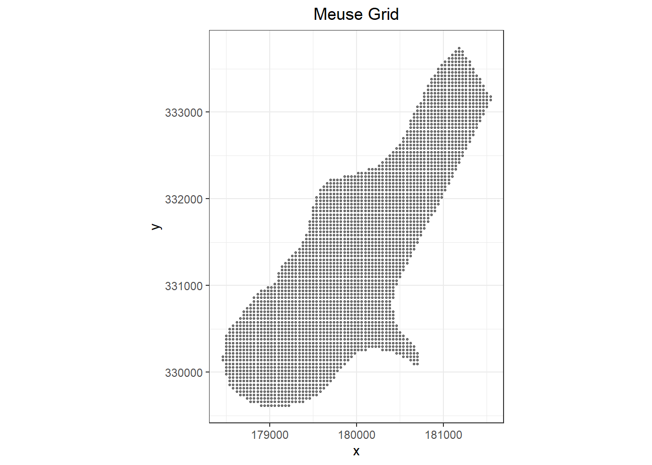
The meuse dataset in the R package sp (Pebesma and Bivand 2005) contains measurements of heavy metals concentrations in topsoil next to the Meuse river, located near the village of Stein in the Netherlands. Heavy metal concentrations are from composite samples of an area of approximately 15 meters by 15 meters. In addition, the meuse.grid dataset includes several of the covariates in the meuse dataset in a regular grid over the study region.
# Load libraries
library(dplyr)
library(gstat)
library(sp)
library(ggplot2)
library(gridExtra)
library(INLA)
library(maptools)

# Funtion for suppressing output
quiet <- function(x) {
  sink(tempfile())
  on.exit(sink())
  invisible(force(x))
}

# Set seed
set.seed(10)

# Load data
data(meuse)
str(meuse)
## 'data.frame':	155 obs. of  14 variables:
##  $ x      : num  181072 181025 181165 181298 181307 ...
##  $ y      : num  333611 333558 333537 333484 333330 ...
##  $ cadmium: num  11.7 8.6 6.5 2.6 2.8 3 3.2 2.8 2.4 1.6 ...
##  $ copper : num  85 81 68 81 48 61 31 29 37 24 ...
##  $ lead   : num  299 277 199 116 117 137 132 150 133 80 ...
##  $ zinc   : num  1022 1141 640 257 269 ...
##  $ elev   : num  7.91 6.98 7.8 7.66 7.48 ...
##  $ dist   : num  0.00136 0.01222 0.10303 0.19009 0.27709 ...
##  $ om     : num  13.6 14 13 8 8.7 7.8 9.2 9.5 10.6 6.3 ...
##  $ ffreq  : Factor w/ 3 levels "1","2","3": 1 1 1 1 1 1 1 1 1 1 ...
##  $ soil   : Factor w/ 3 levels "1","2","3": 1 1 1 2 2 2 2 1 1 2 ...
##  $ lime   : Factor w/ 2 levels "0","1": 2 2 2 1 1 1 1 1 1 1 ...
##  $ landuse: Factor w/ 15 levels "Aa","Ab","Ag",..: 4 4 4 11 4 11 4 2 2 15 ...
##  $ dist.m : num  50 30 150 270 380 470 240 120 240 420 ...
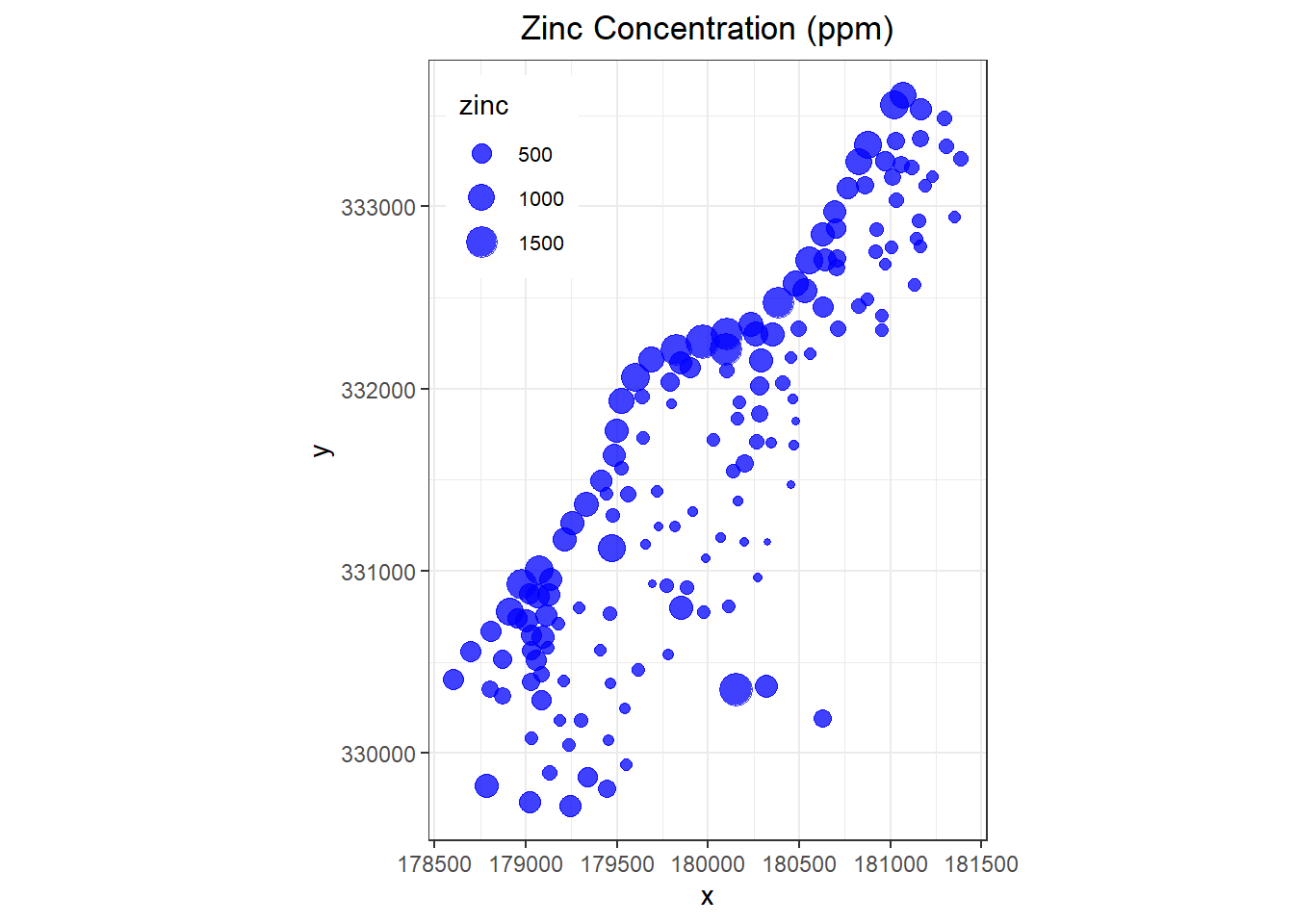
The x and y columns in the dataset are the coordinates of the sample locations using the Rijksdriehoek (RDH) coordinate system. A plot of the meuse.grid is shown below. Also shown below is a bubble plot of zinc concentrations in the topsoil.
# Show grid locations
data(meuse.grid)
ggplot(data = meuse.grid, aes(x, y)) +
  geom_point(size = 0.5, alpha = 0.5) +
  labs(title = 'Meuse Grid') +
  coord_equal() +
  theme_bw() +
  theme(plot.title = element_text(hjust = 0.5))
# Create bubble plot
ggplot(data = meuse, aes(x, y)) +
  geom_point(aes(size = zinc), color = "blue", alpha = 3/4) +
  labs(title = 'Zinc Concentration (ppm)') +
  coord_equal() +
  theme_bw() +
  theme(plot.title = element_text(hjust = 0.5),
        legend.text = element_text(size = 8),
        legend.position = c(0.15, 0.85))
Kriging
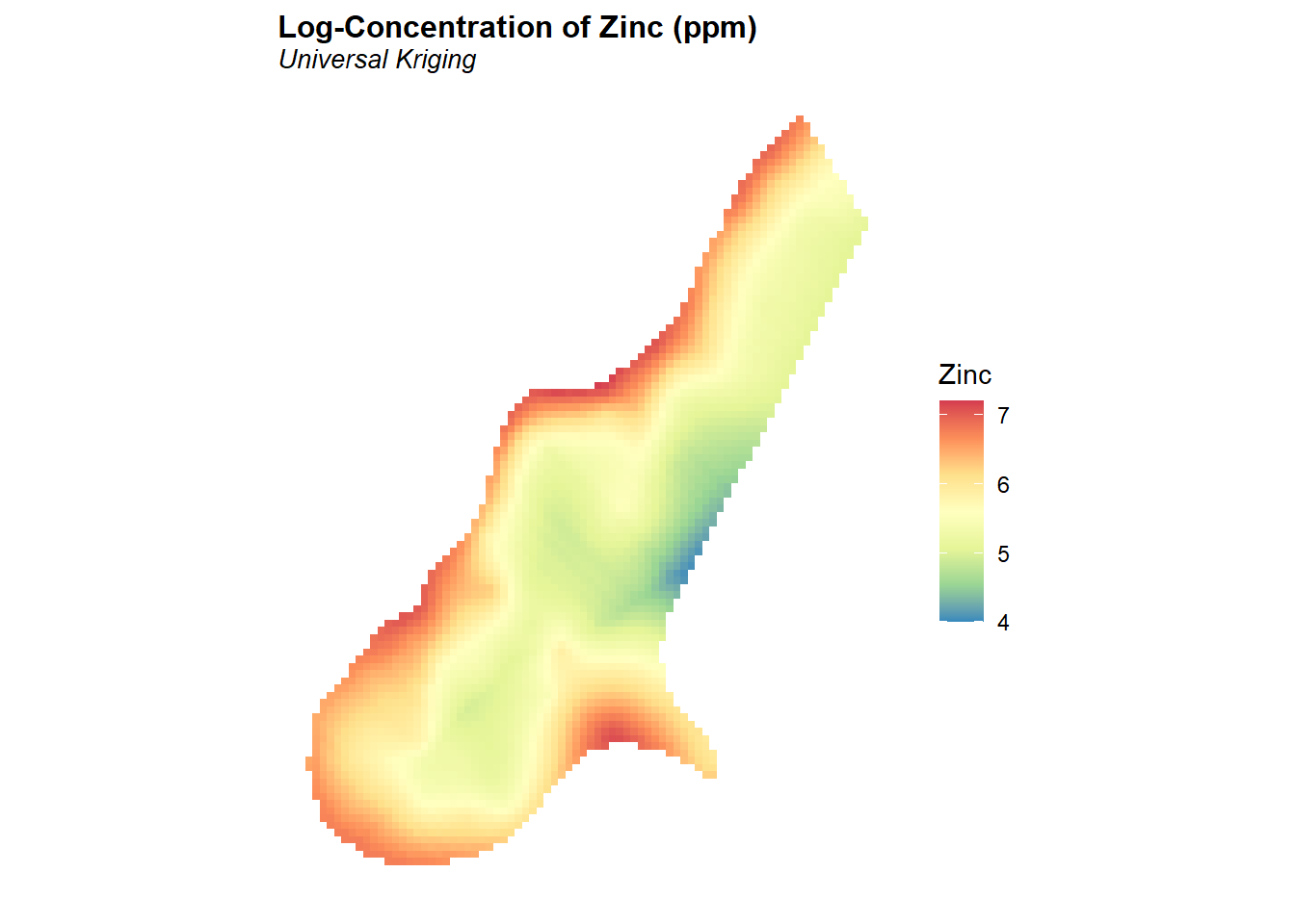
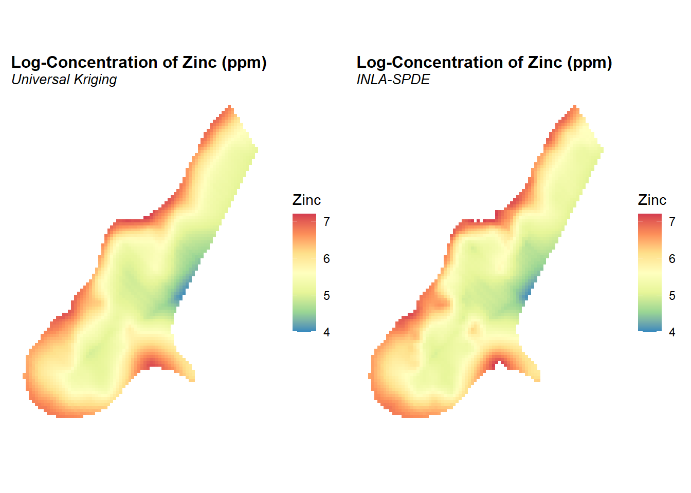
As a preliminary analysis of this dataset, kriging will be used to obtain an estimation of the concentration of zinc at all points of the grid defined in meuse.grid. Universal kriging (Cressie 2015) will be used in order to include covariates in the prediction. For this analysis, normalized distance to the river Meuse is used as a covariate. Kriging is conducted on the natural log of the zinc concentrations. The predicted concentrations of zinc in log-scale are shown in the figure below.
# Create SpatialPointsDataFrame and assign data its coordinate reference system
coordinates(meuse) <- ~x+y
proj4string(meuse) <- CRS("+init=epsg:28992")

# Perform similar operation on the grid
coordinates(meuse.grid) = ~x+y
proj4string(meuse.grid) <- CRS("+init=epsg:28992")
gridded(meuse.grid) = TRUE

# Fit variogram
vgm <- variogram(log(zinc) ~ dist, meuse)
fit.vgm <- fit.variogram(vgm, vgm("Sph"))

# Universal kriging
krg <- quiet(krige(log(zinc) ~ dist, meuse, meuse.grid, model = fit.vgm))

# Add estimates to meuse.grid
meuse.grid$zinc.krg <- krg$var1.pred
meuse.grid$zinc.krg.sd <- sqrt(krg$var1.var)
# Create plot of kriging results
meuse_spdf <- as.data.frame(meuse.grid)
ggplot(meuse_spdf, aes(x = x, y = y, fill = zinc.krg)) +
  geom_tile() +
  scale_fill_distiller('Zinc', palette = 'Spectral',
                       na.value = 'transparent',
                       limits = c(4, 7.2)) +
  labs(title = 'Log-Concentration of Zinc (ppm)',
       subtitle = 'Universal Kriging') +
  coord_equal() +
  theme(plot.title = element_text(margin = margin(b = 2), size = 12,
                                  hjust = 0.0, color = 'black',
                                  face = quote(bold)),
        plot.subtitle = element_text(margin = margin(b = 2), size = 10,
                                    hjust = 0.0, color = 'black',
                                    face = quote(italic)),
        line = element_blank(),
        axis.text = element_blank(),
        axis.title = element_blank(),
        panel.background = element_blank())
INLA-SPDE
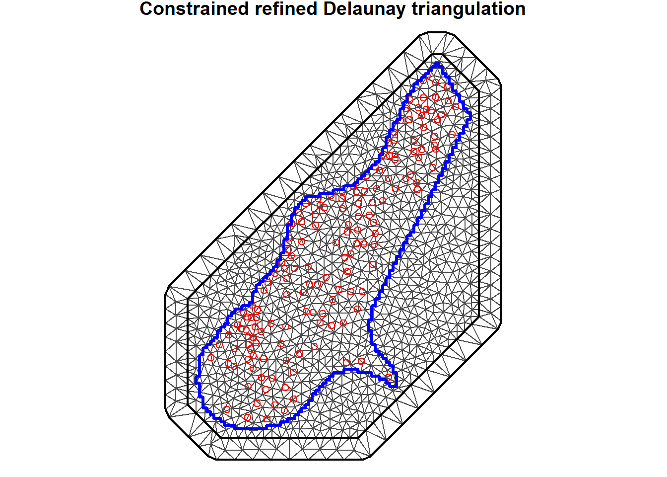
The SPDE approach approximates the continuous Gaussian field as a discrete Gaussian Markov random field by means of a finite basis function defined on a triangulated mesh of the region of study (Moraga 2020). In contrast to ordinary kriging, an irregular grid is used in the prediction process. Observations are treated as initial vertices for the triangulation, and extra vertices are added heuristically to minimize the number of triangles needed to cover the region subject to the triangulation constraints. These extra vertices are used as prediction locations. This partition is usually called mesh. Small triangles are used within the study area, and larger triangles in the extension outside the study area. Triangles in the outer domain are needed to avoid boundary effects. The triangulated mesh obtained is shown below. The blue line represents the meuse.grid boundary and the red circles are the sample locations. A thick line separates the outer offset from the inner offset and the boundary of the study region. The triangulated mesh contains 1,217 vertices.
There are several important aspects of a mesh. The triangle size (determined using a combination of max.edge and cutoff) determines how precisely the equations will be tailored by the data. Using smaller triangles increases precision but also exponentially increases computing power. The edge triangles can be bigger to reduce computing power.
# Boundary
meuse.bdy <- unionSpatialPolygons(
  as(meuse.grid, "SpatialPolygons"), rep (1, length(meuse.grid))
)

# Define mesh
coo <- meuse@coords
pts <- meuse.bdy@polygons[[1]]@Polygons[[1]]@coords
mesh <- inla.mesh.2d(loc.domain = pts, max.edge = c(150, 500),
  offset = c(100, 250))

par(mar = c(0, 0, 0.8, 0))
plot(mesh, asp = 1)
points(coo, col = 'red')
lines(pts, col = 'blue', lwd = 3)
After the mesh has been setup, a projector matrix A is computed. This matrix essentially translates spatial locations on the mesh into vectors in the model. The matrix A has the number of rows equal to the number of observations, and the number of columns equal to the number of vertices of the triangulation (Moraga 2020). The A matrix is combined with the model matrix and random effects in a format called a stack. A summary of the model using this data stack is shown below.
# Create SPDE
meuse.spde <- inla.spde2.matern(mesh = mesh, alpha = 2)
A.meuse <- inla.spde.make.A(mesh = mesh, loc = coordinates(meuse))
s.index <- inla.spde.make.index(name = "spatial.field",
  n.spde = meuse.spde$n.spde)

# Create data structure
meuse.stack <- inla.stack(data  = list(zinc = meuse$zinc),
  A = list(A.meuse, 1),
  effects = list(c(s.index, list(Intercept = 1)),
    list(dist = meuse$dist)),
  tag = "meuse.data")

# Create data structure for prediction
A.pred <- inla.spde.make.A(mesh = mesh, loc = coordinates(meuse.grid))
meuse.stack.pred <- inla.stack(data = list(zinc = NA),
  A = list(A.pred, 1),
  effects = list(c(s.index, list (Intercept = 1)),
    list(dist = meuse.grid$dist)),
  tag = "meuse.pred")

# Join stack
join.stack <- inla.stack(meuse.stack, meuse.stack.pred)

# Fit model
form <- log(zinc) ~ -1 + Intercept + dist + f(spatial.field, model = spde)

m1 <- inla(form, data = inla.stack.data(join.stack, spde = meuse.spde),
  family = "gaussian",
  control.predictor = list(A = inla.stack.A(join.stack), compute = TRUE),
  control.compute = list(cpo = TRUE, dic = TRUE))

# Summary of results
summary(m1)
##
## Call:
##    c("inla(formula = form, family = \"gaussian\", data =
##    inla.stack.data(join.stack, ", " spde = meuse.spde), control.compute =
##    list(cpo = TRUE, dic = TRUE), ", " control.predictor = list(A =
##    inla.stack.A(join.stack), compute = TRUE))" )
## Time used:
##     Pre = 3.3, Running = 25.3, Post = 2.07, Total = 30.7
## Fixed effects:
##             mean    sd 0.025quant 0.5quant 0.975quant   mode kld
## Intercept  6.592 0.140      6.322    6.588      6.881  6.582   0
## dist      -2.812 0.376     -3.561   -2.811     -2.072 -2.808   0
##
## Random effects:
##   Name	  Model
##     spatial.field SPDE2 model
##
## Model hyperparameters:
##                                          mean    sd 0.025quant 0.5quant
## Precision for the Gaussian observations 20.17 7.185       9.33    19.12
## Theta1 for spatial.field                 4.34 0.278       3.79     4.34
## Theta2 for spatial.field                -4.87 0.241      -5.34    -4.88
##                                         0.975quant  mode
## Precision for the Gaussian observations      37.15 17.12
## Theta1 for spatial.field                      4.89  4.34
## Theta2 for spatial.field                     -4.39 -4.89
##
## Deviance Information Criterion (DIC) ...............: 79.15
## Deviance Information Criterion (DIC, saturated) ....: 1903.74
## Effective number of parameters .....................: 91.62
##
## Marginal log-Likelihood:  -107.86
## CPO and PIT are computed
##
## Posterior summaries for the linear predictor and the fitted values are computed
## (Posterior marginals needs also 'control.compute=list(return.marginals.predictor=TRUE)')
According to the fitted model there is a reduction in the concentration of zinc as distance to the river increases. This is consistent with previous findings and the results from the universal kriging.
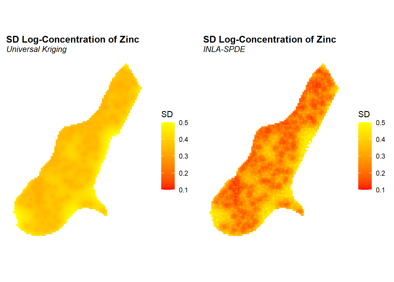
The predicted posterior means of the concentrations of zinc in log-scale and the prediction standard deviations are shown below. The prediction standard deviations are a measure of the uncertainty about the predictions. The point estimates of the concentration seem to be very similar between universal kriging and the model fitted with INLA-SPDE. However, prediction uncertainty seems to be smaller with the INLA-SPDE model. Because we are comparing results from two different inference methods, differences in the uncertainty may be due to the different ways in which the covariance of the spatial effect is computed.
# Get predicted data on grid
index.pred <- inla.stack.index(join.stack, "meuse.pred")$data
meuse.grid$zinc.spde <- m1$summary.fitted.values[index.pred, "mean"]
meuse.grid$zinc.spde.sd <- m1$summary.fitted.values[index.pred, "sd"]

# Plot posterior means using ggplot
meuse_spdf <- as.data.frame(meuse.grid)
p1 <- ggplot(meuse_spdf, aes(x = x, y = y, fill = zinc.krg)) +
  geom_tile() +
  scale_fill_distiller('Zinc', palette = 'Spectral',
                       na.value = 'transparent',
                       limits = c(4, 7.2)) +
  labs(title = 'Log-Concentration of Zinc (ppm)',
       subtitle = 'Universal Kriging') +
  coord_equal() +
  theme(plot.title = element_text(margin = margin(b = 2), size = 12,
                                  hjust = 0.0, color = 'black',
                                  face = quote(bold)),
         plot.subtitle = element_text(margin = margin(b = 2), size = 10,
                                      hjust = 0.0, color = 'black',
                                       face = quote(italic)),
        line = element_blank(),
        axis.text = element_blank(),
        axis.title = element_blank(),
        panel.background = element_blank())

p2 <- ggplot(meuse_spdf, aes(x = x, y = y, fill = zinc.spde)) +
  geom_tile() +
  scale_fill_distiller('Zinc', palette = 'Spectral',
                       na.value = 'transparent',
                       limits = c(4, 7.2)) +
  labs(title = 'Log-Concentration of Zinc (ppm)',
       subtitle = 'INLA-SPDE') +
  coord_equal() +
  theme(plot.title = element_text(margin = margin(b = 2), size = 12,
                                  hjust = 0.0, color = 'black',
                                  face = quote(bold)),
         plot.subtitle = element_text(margin = margin(b = 2), size = 10,
                                      hjust = 0.0, color = 'black',
                                       face = quote(italic)),
        line = element_blank(),
        axis.text = element_blank(),
        axis.title = element_blank(),
        panel.background = element_blank())

grid.arrange(p1, p2, nrow = 1)
# Plot stand deviations using ggplot
p1 <- ggplot(meuse_spdf, aes(x = x, y = y, fill = zinc.krg.sd)) +
  geom_tile() +
  scale_fill_gradient('SD',
                      low = 'red', high = 'yellow',
                      na.value = 'transparent',
                      limits = c(0.1, 0.5)) +
  labs(title = 'SD Log-Concentration of Zinc',
       subtitle = 'Universal Kriging') +
  coord_equal() +
  theme(plot.title = element_text(margin = margin(b = 2), size = 12,
                                  hjust = 0.0, color = 'black',
                                  face = quote(bold)),
         plot.subtitle = element_text(margin = margin(b = 2), size = 10,
                                      hjust = 0.0, color = 'black',
                                       face = quote(italic)),
        line = element_blank(),
        axis.text = element_blank(),
        axis.title = element_blank(),
        panel.background = element_blank())

p2 <- ggplot(meuse_spdf, aes(x = x, y = y, fill = zinc.spde.sd)) +
  geom_tile() +
  scale_fill_gradient('SD',
                      low = 'red', high = 'yellow',
                      na.value = 'transparent',
                      limits = c(0.1, 0.5)) +
  labs(title = 'SD Log-Concentration of Zinc',
       subtitle = 'INLA-SPDE') +
  coord_equal() +
  theme(plot.title = element_text(margin = margin(b = 2), size = 12,
                                  hjust = 0.0, color = 'black',
                                  face = quote(bold)),
         plot.subtitle = element_text(margin = margin(b = 2), size = 10,
                                      hjust = 0.0, color = 'black',
                                       face = quote(italic)),
        line = element_blank(),
        axis.text = element_blank(),
        axis.title = element_blank(),
        panel.background = element_blank())

grid.arrange(p1, p2, nrow = 1)
Conclusion
Many environmental phenomena are monitored over both space and time. Gaussian random fields has become increasingly popular as these data are characterized by a spatial and/or temporal structure which needs to be taken into account in the inferential process. A common challenge when modeling these data is spatio-temporal autocorrelation, whereby observations from geographically close areal units and temporally close time periods tend to have more similar values than units and time periods that are further apart. Although Bayesian inference using MCMC techniques are commonly used, this can be a challenge due to convergence problems and heavy computational loads. Computational issues can arise when working with big dense covariance matrices that occur when large spatio-temporal datasets are analyzed.
The example presented in this Stats Factsheet illustrates an effective spatial prediction strategy for spatio-temporal modeling. The joint use of the SPDE approach together with the INLA algorithm is a powerful technique in overcoming the computational issues related to Gaussian process modeling. This kind of approach is widely used in air pollution studies due to its inextricabity in modeling the effect of relevant covariates (i.e., meteorological and geographical variables) as well as time and space dependence (Cocchi et al. 2007; Cameletti et al. 2011; Sahu 2011; Cameletti et al. 2013; Forlani et al. 2020). Extending spatial applications to space-time is straightforward using INLA-SPDE, as purely temporal random effects can be added to the linear predictor, and the model can be extended to a space-time interaction.
References
Cameletti M., R. Ignaccolo, and S. Bande. 2011. Comparing spatio-temporal models for particulate matter in piemonte. Environmetrics 22, 985-996.
Cameletti M., F. Lindgren, D. Simpson, and H. Rue. 2013. Spatio-temporal modeling of particulate matter concentration through the SPDE approach. AStA Adv Stat Anal 97, 109-131.
Cocchi D, F. Greco, and C. Trivisano. 2007. Hierarchical space-time modelling of PM10 pollution. Atmospheric Environment 41, 532-542.
Cressie, N. 2015. Statistics for Spatial Data. Hoboken, New Jersey, John Wiley & Sons, Inc.
Deutsch C.V. and A.G. Journel. 1998. *GSLIB Geostatistical Software Library and User’s Guide, Second Edition.*New York, Oxford University Press.
C. Forlani, S. Bhatt, M. Cameletti, E. Krainski, and M. Blangiardo. 2020. A joint Bayesian space-time model to integrate spatially misaligned air pollution data in R‐INL.Environmetrics 3::e2644. 1-17.
Lindgren, F., H. Rue, and J. Lindström. 2011. An Explicit Link Between Gaussian Fields and Gaussian Markov Random Fields: The Stochastic Partial Differential Equation Approach (with Discussion). Journal of the Royal Statistical Society: Series B 73, 423-98.
Lindgren, F. and H. Rue. 2015. Bayesian Spatial Modelling with R-INLA. Journal of Statistical Software 63. https://doi.org/10.18637/jss.v063.i19.
Martino, S. and A. Riebler. 2019. Integrated Nested Laplace Approximations (INLA). https://arxiv.org/abs/1907.01248.
Matheron, G. 1963 Principles of Geostatistics. Economic Geology, 58, 1246-1266.
Moraga, P. 2020. Geospatial Health Data: Modeling and Visualization with R-INLA and Shiny. Boca Raton, CRC Press.
Pebesma, E.J. and R.S. Bivand. 2005. Classes and methods for spatial data in R. R News, 5.
Rue, H., S. Martino, and N. Chopin. 2009. Approximate Bayesian inference for latent Gaussian models by using integrated nested Laplace approximations. Journal of the Royal Statistical Society: Series B, 71, 319-392.
Sahu S. 2011. Hierarchical Bayesian models for space-time air pollution data. In: Rao C (ed), Handbook of Statistics - Time Series Analysis, Methods and Applications, Handbook of Statistics, Vol 30, Holland, Elsevier Publishers.
Williams, C. K. I. 1998. Prediction with Gaussian Processes: From Linear Regression to Linear Prediction and Beyond. Learning in Graphical Models, 599-621.
Yang, X., G. Tartakovsky, and A. Tartakovsky. 2018. Physics-Informed Kriging: A Physics-Informed Gaussian Process Regression Method for Data-Model Convergence. ISE Technical Report 19T-026, Lehigh University.
- Posted on:
- January 19, 2021
- Length:
- 16 minute read, 3296 words
- See Also: