Spatio-temporal Modeling of PM10 Concentration Using INLA-SPDE
By Charles Holbert
January 20, 2021
# Load libraries
library(INLA)
library(lattice)
library(abind)
library(fields)    # for the color palette
library(splancs)   # fof selecting points inside Piemonte

# Load covariates selector file
source("./data/Covariates/covariates_selector.R")

# Set seed
set.seed(10)
Introduction
This example illustrates how a stochastic partial differential equation (SPDE) approach with Integrated Nested Laplace Approximation (INLA) can be used for modeling the spatio-temporal behavior of particulate matter \((PM_{10})\) concentrations measured in the North-Italian region of Piemonte. The model involves a Gaussian Field (GF), affected by a measurement error, and a state process characterized by a first order autoregressive dynamic model and spatially correlated covariates. The objective of the model is to predict air pollution for a given day in the Piemonte region. In addition, a map will be generated showing the probability of exceeding the 50 \(µg/m^3\) threshold value. Note that this case study has been described in Cameletti et al. (2011), but is being presented here as a tutorial in spatial and spatio-temporal modeling using R-INLA.
Data
During October 2005 to March 2006, \(PM_{10}\) concentrations given in in \(µg/m^3\) were measured in the North-Italian region of Piemonte at 24 air monitoring stations. Cameletti et al. (2011) provide a description of the PM10 data as well as the covariates recorded at each station, including daily maximum mixing height (HMIX, in m), daily total precipitation (PREC, in mm), daily mean wind speed (WS, in m/s), daily mean temperature (TEMP, in K), daily emission rates of primary aerosols (EMI, in g/s), altitude (A, in m) and spatial coordinates (UTMX and UTMY in km).
# Load the data for the 24 stations and 182 days
Piemonte_data <- read.table(
  "./data/Piemonte_data_byday.csv",
  header = TRUE, sep = ","
)
str(Piemonte_data)
## 'data.frame':	4368 obs. of  11 variables:
##  $ Station.ID: int  1 2 3 4 5 6 7 8 9 10 ...
##  $ Date      : chr  "01/10/05" "01/10/05" "01/10/05" "01/10/05" ...
##  $ A         : num  95.2 164.1 242.9 149.9 405 ...
##  $ UTMX      : num  469 423 491 437 426 ...
##  $ UTMY      : num  4973 4951 4949 4973 5046 ...
##  $ WS        : num  0.9 0.82 0.96 1.17 0.6 1.02 1.09 0.9 0.64 0.81 ...
##  $ TEMP      : num  289 289 287 289 288 ...
##  $ HMIX      : num  1295 1140 1404 1042 1039 ...
##  $ PREC      : num  0 0 0 0 0 0 1.05 0 0 0 ...
##  $ EMI       : num  26.05 18.74 6.28 29.35 32.19 ...
##  $ PM10      : int  28 22 17 25 20 41 17 18 33 23 ...
Let’s load the file containing the spatial coordinates for each air monitoring station and the boundary of the Piemonte region.
# Load coordinate file
coordinates <- read.table(
  "./data/coordinates.csv",
  header = TRUE, sep = ","
)
rownames(coordinates) <- coordinates[,"Station.ID"]

# Get borders of Piemonte (in km)
borders <-read.table(
  "./data/Piemonte_borders.csv",
  header = TRUE, sep = ",")
Finally, let’s load the covariate arrays and the Piemonte grid file.
# Load the covariate arrays (each array except for A is 56x72x182)
load("./data/Covariates/Altitude_GRID.Rdata")     # A; Altitude GRID
load("./data/Covariates/WindSpeed_GRID.Rdata")    # WS; WindSpeed GRID
load("./data/Covariates/HMix_GRID.Rdata")         # HMIX; HMixMax GRID
load("./data/Covariates/Emi_GRID.Rdata")          # EMI; Emi GRID
load("./data/Covariates/Temp_GRID.Rdata")         # TEMP; Mean_Temp
load("./data/Covariates/Prec_GRID.Rdata")         # PREC; Prec

# Load the Piemonte grid c(309, 529), c(4875, 5159), dims = c(56, 72)
load("./data/Covariates/Piemonte_grid.Rdata")
The data are composed of 24 stations, 4,368 space-time events, and 182 time points.
# Get number of stations and data
n_stations <- length(coordinates$Station.ID)    # 24 stations
n_data <- length(Piemonte_data$Station.ID)      # 4368 space-time data
n_days <- n_data/n_stations                     # 182 time points
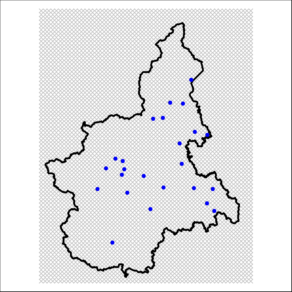
Let’s create a plot of the Piemonte region grid with the air monitoring stations.
par(mar = c(0, 0, 0, 0))
plot(
  Piemonte_grid,
  col = "grey", pch = 4, asp = 1,
  xlim = range(Piemonte_grid$UTMX_km)
)
lines(borders, lwd = 3, asp = 1)
points(coordinates$UTMX, coordinates$UTMY, pch = 20, cex = 1.4, col = "blue")
To stabilize the variance, which increases with the mean values, and to make the distribution of PM10 data approximately normal, we use a logarithmic transformation and add a new variable named logPM10 to the Piemonte data.
Piemonte_data$logPM10 <- log(Piemonte_data$PM10) # 182 time points
The ranges of the covariates are significantly different. When using covariates that have different units of measure and different variances, the data need to be standardized. Thus, the covariate data are standardized by mean-centering and scaling to unit variance prior to analysis.
mean_covariates <- apply(Piemonte_data[,3:10], 2, mean)
sd_covariates <- apply(Piemonte_data[,3:10], 2, sd)
Piemonte_data[,3:10] <- scale(
  Piemonte_data[,3:10],
  center = mean_covariates,
  scale = sd_covariates
)
To simplify keeping track of the temporal aspect of the data, time is added as the index of each observation day.
Piemonte_data$time <- rep(1:n_days, each = n_stations)
A matrix of station ids and coordinates is created for later use.
coordinates.allyear <- as.matrix(
  coordinates[Piemonte_data$Station.ID, c("UTMX", "UTMY")]
)
dim(coordinates.allyear)
## [1] 4368 2
Prediction Day
Let’s pick day number 122 for our predictions.
# Extract the standardized covariate for day i_day (you get a 56x72x8 matrix)
i_day <- 122
which_date <- unique(Piemonte_data$Date)[i_day]
print(paste("**---- You will get a prediction for ", which_date, "---**"))
## [1] "**---- You will get a prediction for 30/01/06 ---**"
# Standardise the covariates for the selected day
covariate_array_std <- covariates_selector_funct(
  i_day, mean_covariates, sd_covariates
)
Let’s assign altitude values greater than 7 (1 km) a value of NA.
elevation <- covariate_array_std[,,1]
index_mountains <- which(elevation > 7)
elevation[elevation > 7] <- NA
covariate_array_std[,,1] <- elevation
Let’s reshape the 3D array (56x72x8) into a data frame (4032x8) with the 8 covariates on the columns.
covariate_matrix_std <- data.frame(
  apply(covariate_array_std, 3, function(X) c(t(X)))
)
colnames(covariate_matrix_std) <- colnames(Piemonte_data[,3:10])
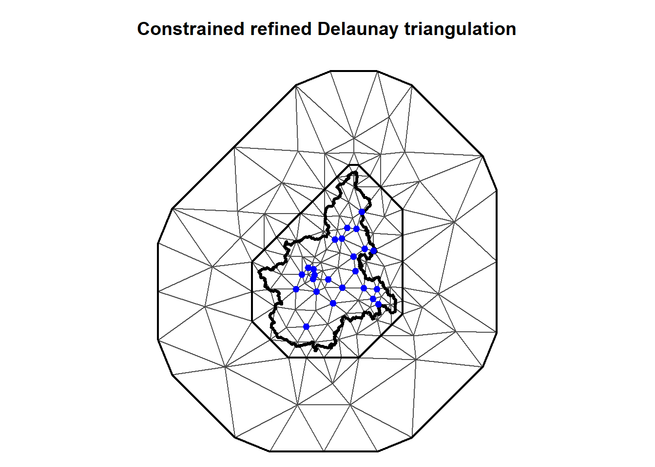
Triangulation
We triangulate the Piemonte region using the built-in inla.mesh.2d function. A triangulation of the domain is created that is defined by the region border, using a convex set with 8 edges at a distance of 10 km. To reduce boundary effects of the SPDE, a further extension with 16 edges is added at a distance of 140 km, giving a total extension of 150 km. The maximal edge length is specified as 50 km in the interior of the region, and 1,000 km in the outer extension. Since the outer extension is of no practical interest, the resolution needs only to be as fine as required by the numerics. In this case, the boundary effect can be handled well by only specifying the minimal allowed interior angle for the triangles, with 21 degrees being the largest number guaranteeing termination of the triangulation algorithm. Using 26 degrees for the inner region and 21 degrees for the outer extension, the number of vertices becomes 142 (stored in mesh$n).
Piemonte_mesh <- inla.mesh.2d(
  loc = cbind(coordinates$UTMX, coordinates$UTMY),
  loc.domain = borders,
  offset = c(10, 140),
  max.edge = c(50, 1000),
  min.angle = c(26, 21),
  cutoff = 0,
  plot.delay = NULL
)
Let’s create a plot of the triangulation covering the Piemonte region and stretching out towards the extended boundary.
par(mar = c(0, 0, 3, 0))
plot(Piemonte_mesh, asp = 1)
lines(borders, lwd = 3)
points(
  coordinates$UTMX, coordinates$UTMY,
  pch = 20, cex = 1.4, col = "blue"
)
Model
SPDE Object
Now, we will create a SPDE model object for a Matérn spatial covariance function specifying the triangulation (given by the mesh object) and the parameter \(\alpha\) = 2. Parameter \(\alpha\) is related to the smoothness parameter of the process, namely, \(\alpha\) = v + d/2. In this example, we set the smoothness parameter equal to 1 and so \(\alpha\) = 1 + 2 / 2 = 2.
Piemonte_spde <- inla.spde2.matern(
  mesh = Piemonte_mesh,
  alpha = 2
)
Index Sets
The observation models allows us to simplify specification of the latent model through the helper function inla.spde.make.index, which generates vectors of indices for the spatial and temporal components of the model. We specify the name of the effect(s) and the number of vertices in the SPDE model (spde$n.spde).
s_index <- inla.spde.make.index(
  name = "spatial.field",
  n.spde = Piemonte_spde$n.spde,
  n.group = n_days
)
names(s_index)
## [1] "spatial.field" "spatial.field.group" "spatial.field.repl"
A Matrices
Now, we construct an observation matrix that extracts the values of the spatio-temporal field at the measurement locations and time points used for the parameter estimation. This is a projection matrix A used to project the Gaussian random field (GRF) from the observations to the triangulation vertices.
# Create A matrix for the estimation part
A_est <- inla.spde.make.A(
  mesh = Piemonte_mesh,
  loc = coordinates.allyear,
  group = Piemonte_data$time,
  n.group = n_days
)
dim(A_est)
## [1] 4368 25844
# Create A matrix for grid prediction of day number i_day
A_pred <- inla.spde.make.A(
  mesh=  Piemonte_mesh,
  loc = as.matrix(Piemonte_grid),
  group = i_day,                   # selected day for prediction
  n.group = n_days
)
dim(A_pred)
## [1] 4032 25844
Stacks
We will use the inla.stack function to organize the data, effects, and projection matrices. We construct a stack with data for estimation and tag it with the string “est”. We also construct a stack for prediction and tag it with “pred.” The response vector is set to NA, and the data is specified at the prediction locations. Finally, we put estimation and prediction stacks together in a full stack.
In each inla.stack call, effects is a list of linear predictor component groups, such that each group has its own observation matrix, specified as the list of matrices A, with 1 interpreted as an identity matrix. The result is a linear predictor model with the sum of the observed component groups as its final value, as well as predictors for the validation stations and a joint predictor for all the spatial components on the given prediction day.
# Estimation stack
stack_est <- inla.stack(
  data = list(logPM10 = Piemonte_data$logPM10),
  A = list(A_est, 1),
  effects = list(
    c(s_index, list(Intercept = 1)),
    list(Piemonte_data[,3:10])
  ),
  tag = "est"
)

# Prediction stack
stack_pred <- inla.stack(
  data = list(logPM10 = NA),
  A = list(A_pred, 1),
  effects = list(
    c(s_index,list(Intercept = 1)),
    list(covariate_matrix_std)
  ),
  tag = "pred"
)

# Final stack containing the estimation and prediction stacks
stack <- inla.stack(stack_est, stack_pred)
Formula
We specify the linear predictor model as an R-INLA formula object. This includes the covariates (fixed effects) together with random effect components, specified by the f(.) function, which is designed to define non-fixed effects such as spatial random effects, time trends, seasonal effects, etc. With the following specification of f(.), through the group and control.group options, we specify that, at each time point, the spatial locations are linked by the SPDE model object, while across time, the process evolves according to an AR(1) process.
The formula is specified by including the response in the left-hand side, and the fixed and random effects in the right-hand side. In the formula we remove the intercept (adding 0) and add it as a covariate term (adding b0).
formula <- logPM10 ~ -1 + Intercept + A + UTMX + UTMY + WS + TEMP + HMIX + PREC + EMI +
  f(spatial.field,
    model = Piemonte_spde,
    group = spatial.field.group,
    control.group = list(model = "ar1")
  )
Model Results
The specified model with Gaussian response can be run calling the inla function.
# ATTENTION: the run is computationally intensive!

output <- inla(
  formula,
  data = inla.stack.data(stack, spde = Piemonte_spde),
  family = "gaussian",
  control.predictor = list(A = inla.stack.A(stack), compute = TRUE),
  control.compute = list(return.marginals.predictor = TRUE),
  control.inla = list(reordering = "metis"),
  keep = FALSE, verbose = FALSE
)
print(summary(output))
##
## Call:
##    c("inla(formula = formula, family = \"gaussian\", data =
##    inla.stack.data(stack, ", " spde = Piemonte_spde), verbose = FALSE,
##    control.compute = list(return.marginals.predictor = TRUE), ", "
##    control.predictor = list(A = inla.stack.A(stack), compute = TRUE), ", "
##    control.inla = list(reordering = \"metis\"), keep = FALSE)" )
## Time used:
##     Pre = 3.98, Running = 790, Post = 4.58, Total = 799
## Fixed effects:
##             mean    sd 0.025quant 0.5quant 0.975quant   mode kld
## Intercept  3.687 0.453      2.782    3.689      4.580  3.692   0
## A         -0.199 0.050     -0.299   -0.199     -0.100 -0.198   0
## UTMX      -0.158 0.163     -0.482   -0.157      0.160 -0.155   0
## UTMY      -0.184 0.150     -0.483   -0.184      0.112 -0.183   0
## WS        -0.060 0.008     -0.076   -0.060     -0.043 -0.060   0
## TEMP      -0.119 0.035     -0.188   -0.119     -0.050 -0.119   0
## HMIX      -0.024 0.013     -0.050   -0.024      0.001 -0.024   0
## PREC      -0.054 0.009     -0.070   -0.054     -0.037 -0.054   0
## EMI        0.038 0.015      0.009    0.038      0.067  0.038   0
##
## Random effects:
##   Name	  Model
##     spatial.field SPDE2 model
##
## Model hyperparameters:
##                                           mean    sd 0.025quant 0.5quant
## Precision for the Gaussian observations 30.503 0.861     28.733   30.537
## Theta1 for spatial.field                 3.183 0.049      3.078    3.186
## Theta2 for spatial.field                -4.591 0.043     -4.681   -4.589
## GroupRho for spatial.field               0.961 0.006      0.948    0.961
##                                         0.975quant   mode
## Precision for the Gaussian observations     32.125 30.669
## Theta1 for spatial.field                     3.274  3.196
## Theta2 for spatial.field                    -4.512 -4.580
## GroupRho for spatial.field                   0.973  0.961
##
## Marginal log-Likelihood:  -463.38
## Posterior summaries for the linear predictor and the fitted values are computed
## (Posterior marginals needs also 'control.compute=list(return.marginals.predictor=TRUE)')
Posterior Summaries
The posterior summary statistics (mean, quantiles and standard deviations) of the fixed effects (i.e., the beta covariate coefficients), are obtained from output$summary.fixed.
# Fixed effects betas
fixed.out <- round(output$summary.fixed, 3)
fixed.out
##             mean    sd 0.025quant 0.5quant 0.975quant   mode kld
## Intercept  3.687 0.453      2.782    3.689      4.580  3.692   0
## A         -0.199 0.050     -0.299   -0.199     -0.100 -0.198   0
## UTMX      -0.158 0.163     -0.482   -0.157      0.160 -0.155   0
## UTMY      -0.184 0.150     -0.483   -0.184      0.112 -0.183   0
## WS        -0.060 0.008     -0.076   -0.060     -0.043 -0.060   0
## TEMP      -0.119 0.035     -0.188   -0.119     -0.050 -0.119   0
## HMIX      -0.024 0.013     -0.050   -0.024      0.001 -0.024   0
## PREC      -0.054 0.009     -0.070   -0.054     -0.037 -0.054   0
## EMI        0.038 0.015      0.009    0.038      0.067  0.038   0
The summary statistics of the posterior distribution of the AR(1) coefficient a are obtained from output$summary.hyperparmatrix.
# Hyperparameters sigma2eps and AR(1)
rownames(output$summary.hyperpar)
## [1] "Precision for the Gaussian observations"
## [2] "Theta1 for spatial.field"
## [3] "Theta2 for spatial.field"
## [4] "GroupRho for spatial.field"
As we are interested in the variance \(\sigma_e^2\), we need to transform the marginal density of the precision using the inla.tmarginal function.
sigma2e_marg <- inla.tmarginal(function(x) 1/x, output$marginals.hyperpar[[1]])
Using the inla.emarginal and inla.eqmarginal functions, we can compute the mean, the standard deviation, and the quantiles of \(\sigma_e^2\).
sigma2e_m1 <- inla.emarginal(function(x) x, sigma2e_marg)
sigma2e_m2 <- inla.emarginal(function(x) x^2, sigma2e_marg)
sigma2e_stdev <- sqrt(sigma2e_m2 - sigma2e_m1^2)
sigma2e_quantiles <- inla.qmarginal(c(0.025, 0.5, 0.975), sigma2e_marg)
The AR(1) parameter is given by:
ar <- output$summary.hyperpar["GroupRho for spatial.field",]
Posterior estimates for \(\sigma_C^2\) and r can be obtained by applying the inla.spde2.result function.
# Spatial parameters sigma2 and range
mod.field <- inla.spde2.result(
  output,
  name = "spatial.field",
  Piemonte_spde
)

# sigma2omega
var.nom.marg <- mod.field$marginals.variance.nominal[[1]]
var.nom.m1 <- inla.emarginal(function(x) x, var.nom.marg)
var.nom.m2 <- inla.emarginal(function(x) x^2, var.nom.marg)
var.nom.stdev <- sqrt(var.nom.m2 - var.nom.m1^2)
var.nom.quantiles <- inla.qmarginal(c(0.025, 0.5, 0.975), var.nom.marg)

# Range
range.nom.marg <- mod.field$marginals.range.nominal[[1]]
range.nom.m1 <- inla.emarginal(function(x) x, range.nom.marg)
range.nom.m2 <- inla.emarginal(function(x) x^2, range.nom.marg)
range.nom.stdev <- sqrt(range.nom.m2 - range.nom.m1^2)
range.nom.quantiles <- inla.qmarginal(c(0.025, 0.5, 0.975), range.nom.marg)

# Get the posterior mean values
index_pred <- inla.stack.index(stack,"pred")$data
lp_marginals <- output$marginals.linear.predictor[index_pred]

lp_mean <- unlist(lapply(lp_marginals, function(x) inla.emarginal(exp, x)))
lp_grid_mean <- matrix(lp_mean, 56, 72, byrow = T)
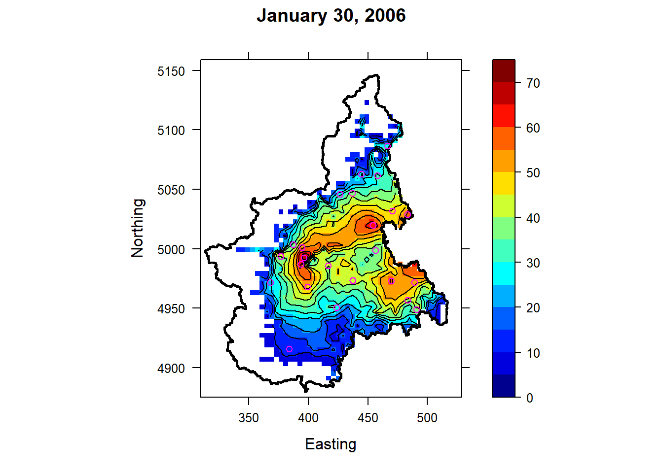
Prediction and Probability of Exceedance Maps
First, we need to select only the points inside the Piemonte region using the splancs library. Points outside the region will be assigned a value of NA.
lp_grid_mean[index_mountains] <- NA
inside_Piemonte <- matrix(inout(Piemonte_grid, borders), 56, 72, byrow = T)
inside_Piemonte[inside_Piemonte == 0] <- NA
inside_lp_grid_mean <- inside_Piemonte * lp_grid_mean
Let’s create a map for January 30, 2006 of the \(PM_{10}\) posterior mean using the levelplot function of the lattice library using the color palette tim.colors contained in the fields library. Note that only locations with an altitude below 1 km are shown.
seq.x.grid <- seq(
  range(Piemonte_grid[,1])[1],
  range(Piemonte_grid[,1])[2],
  length = 56
)

seq.y.grid <- seq(
  range(Piemonte_grid[,2])[1],
  range(Piemonte_grid[,2])[2],
  length = 72
)

# Create prediction map
print(
  levelplot(
    x = inside_lp_grid_mean,
    row.values = seq.x.grid,
    column.values = seq.y.grid,
    ylim = c(4875, 5159),
    xlim = c(309, 529),
    col.regions = fields::tim.colors(64),  # gray(seq(0.9, 0.2, l = 100)),
    aspect = "iso",
    contour = TRUE,
    labels = FALSE,
    pretty = TRUE,
    xlab = "Easting", ylab = "Northing",
    main = format(as.Date(as.character(which_date), '%d/%m/%y'), '%B %d, %Y')
  )
)
trellis.focus("panel", 1, 1, highlight = FALSE)
lpoints(borders, col = 1, cex = 0.25)
## NULL
lpoints(coordinates$UTMX, coordinates$UTMY, col = "magenta", lwd = 1, pch = 21)
## NULL
trellis.unfocus()
Now, let’s a map showing the probability of \(PM_{10}\) concentrations exceeding the 50 \(µg/m^3\) threshold value for January 30, 2006. Note that only locations with an altitude below 1 km are shown.
# Calculate probability of exceedance
threshold <- log(50)
prob  <- lapply(X = lp_marginals, FUN = function(x) inla.pmarginal(marginal = x,threshold))
tailprob_grid <- matrix(1 - unlist(prob), 56, 72, byrow = T)
tailprob_grid[index_mountains] <- NA
inside_tailprob_grid <- inside_Piemonte * tailprob_grid

# Create exceedance probalility map
print(
  levelplot(
    x = inside_tailprob_grid,
    row.values = seq.x.grid,
    column.values = seq.y.grid,
    ylim = c(4875, 5159),
    xlim = c(309, 529),
    at = seq(0, 1, by = 0.1),
    col.regions = fields::tim.colors(64),  # gray(seq(0.9, 0.2, l = 100)),
    aspect = "iso",
    contour = TRUE,
    labels = FALSE,
    pretty = TRUE,
    xlab = "Easting", ylab = "Northing",
    main = format(as.Date(as.character(which_date), '%d/%m/%y'), '%B %d, %Y')
  )
)
trellis.focus("panel", 1, 1, highlight = FALSE)
lpoints(borders, col = 1, cex = 0.25)
## NULL
lpoints(coordinates$UTMX, coordinates$UTMY, col = "magenta", lwd = 1, pch = 21)
## NULL
trellis.unfocus()
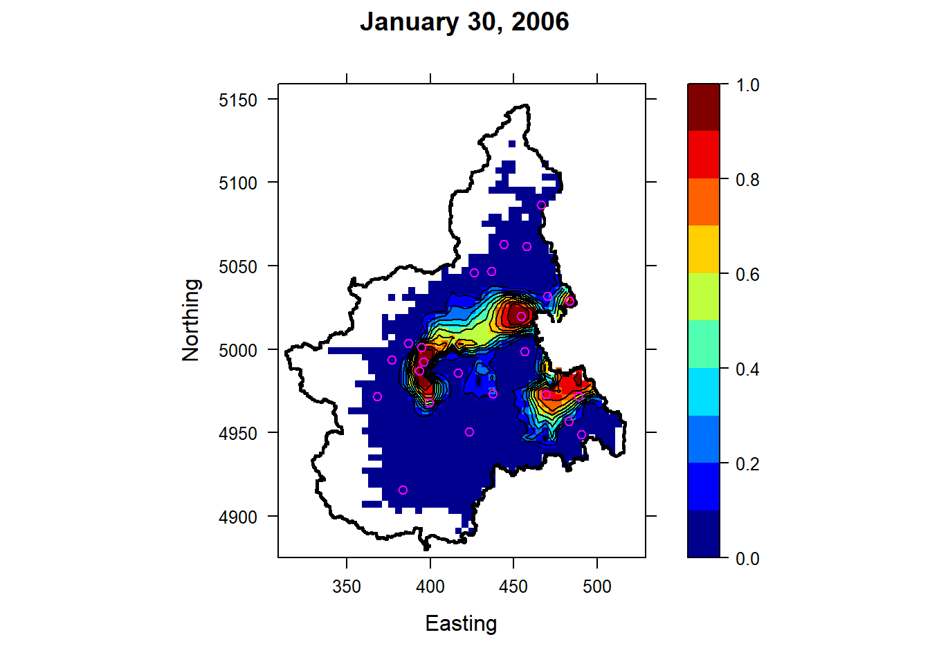
Higher levels of \(PM_{10}\) pollution and exceedance probabilities are associated with the metropolitan areas located near the main cities of the region (Torino, Vercelli, and Novara) and moving eastwards toward Milan.
References
Cameletti M., R. Ignaccolo, and S. Bande. 2011. Comparing spatio-temporal models for particulate matter in piemonte. Environmetrics 22, 985-996.
- Posted on:
- January 20, 2021
- Length:
- 14 minute read, 2893 words
- See Also: