Temporal Optimization of Groundwater Sample Frequency Using Iterative Thinning
By Charles Holbert
March 11, 2021
Introduction
Optimization of groundwater monitoring well networks includes both spatial optimzation and temporal optimization. Temporal optimization is concerned with identifying an optimal frequency of sample collection. In contrast to spatial optimization, temporal analysis is not designed to determine which well locations might be redundant and perhaps unnecessary to the monitoring program. Rather, the goal of temporal optimization is to examine and optimize well sampling frequencies for currently existing locations.
The frequency of sampling necessary to achieve the temporal objective of monitoring can be based on trend detection, accuracy of estimation of periodic fluctuations, or accuracy of estimation of long-term average concentrations. A method that can be used to determine sample frequency is based on an analysis of historical concentration trends that can be reconstructed when sampling events are iteratively removed from the monitoring program. The minimum frequency of past sampling events that can re-produce the same general concentration trend that has been observed when using all sampling events is used as a basis for the recommended future sample frequency. This approach is referred to as “Iterative Thinning.” Because each well is analyzed separately, it is quite possible to have a different recommended sampling interval for each well after applying the Iterative Thinning routine. However, the optimized sampling intervals can be analyzed as a whole and the median optimal sampling interval determined for all monitoring wells or a subset of those wells.
Procedure
The Iterative Thinning approach presented in this Stats Factsheet is based on an algorithm published by Cameron (2004). Iterative Thinning also is used in the Visual Sample Plan (VSP) software (PNNL 2014) and AFCEE’s Geostatistical Temporal-Spatial (GTS) groundwater optimization software (ESTCP 2010) to evaluate monitoring well sampling frequency. The objective of the algorithm is to identify the frequency of sampling required to reproduce the temporal trend of the full dataset.
The following steps are used to optimize the sampling frequency for a given well and constiutent using the Iterative Thinning approach:
-
Determine the current average sampling interval using the existing, historical data.
-
Fit a trend to these initial data along with statistical confidence intervals around the trend.
-
Iteratively remove, at random, certain fractions of the original data.
-
Re-estimate the trend based on the reduced dataset to determine whether the trend still lies within the original confidence bounds.
-
If too much of the new trend falls outside the confidence intervals, stop removing data and compute a new, optimized sampling interval based on the remaining observations.
The mean temporal sample spacing between historical observations is calculated and used as the baseline sample frequency. The Iterative Thinning algorithm uses local polynomial regression (Loader 1999) to fit a smooth trend and confidence intervals around data from the full temporal monitoring record. A percentage of the data points are removed from the dataset and local polynomial regression is used with the same bandwidth to fit a smooth trend to the reduced dataset. The ability of the reduced dataset to reproduce the temporal trends in the full dataset is evaluated by calculating the percentage of the data points on the trend for the reduced dataset that fall within the confidence interval established using the full dataset. Increasing numbers of data points are removed from the dataset and each of the reduced datasets is evaluated for their ability to reproduce the trend observed in the full dataset. A stopping point is reached when too much of the re-estimated trend falls outside the limits of the confidence interval.
Local polynomial regression can be sensitive to the bandwidth used in the regression. If the bandwidth is too small, insufficient data fall within the smoothing window, resulting in a large variance. On the other hand, if the bandwidth is too large, the local polynomial may not fit the data well within the smoothing window, and important features of the mean function may be distorted or lost completely. That is, the fit will have large bias. The bandwidth should be chosen to compromise this bias-variance trade-off. Additionally, the confidence interval is calculated as a simultaneous confidence interval. Whereas a point-wise confidence interval is calculated independently for each observation, ignoring the presence of the other observations, a simultaneous confidence interval is calculated for all observations and provides the stated coverage for the entire line.
To reduce artifacts that might arise from removing a single set of data, the iterative removal process is repeated hundreds of times using randomly selected points from the entire dataset. The proportion of data that can be removed while still reproducing the temporal trend of the full data is used to estimate an optimal sampling frequency.
Parameters
Several libraries and custom functions are required to perform the iterative thinning. Parameters used for this example include a nearest-neighbor-based bandwidth covering 75% of the data; a 90% simultaneous confidence interval established using the full dataset; and an acceptability level of 75%. The iterative removal process will be repeated 200 times using randomly selected points from the entire dataset.
# Load libraries
library(dplyr)
library(lubridate)
library(ggplot2)
library(grid)
library(locfit)

# Load functions
source('functions/annotation_ticks.R')
source('functions/get_loess.R')
source('functions/SumStats.R')

# Set theme for ggplots
theme_set(theme_bw())

# Funtion for suppressing output
quiet <- function(x) {
  sink(tempfile())
  on.exit(sink())
  invisible(force(x))
}

# Set initial values
span <- 0.75
conf <- 0.90
nmsh <- 100
limit <- 0.75
nreps <- 200
Data
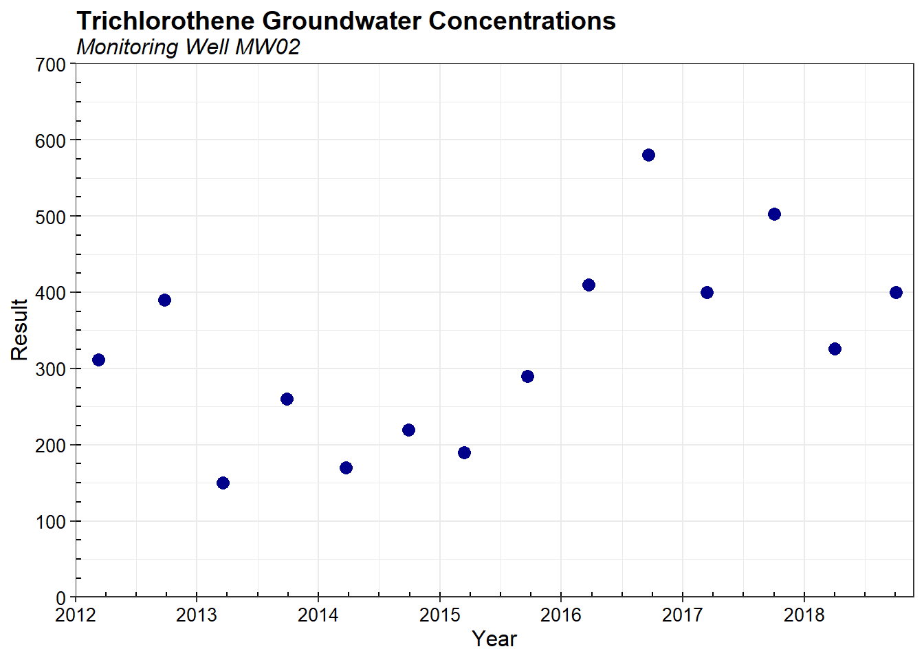
For this example, the data consist of trichloroethene concentrations measured in groundwater at a single monitoring well MW02. Sampling was conducted between March 2012 and October 2018. Descriptive statistics are provided below and include the total number of samples, detected results, and frequency of detection; the minimum and maximum concentrations for detected and non-detected observations; and the mean, median, standard deviation (SD), and coefficient of variation (CV). Concentrations are given in micrograms-per-liter (µg/L).
# Read comma-delimited file
dat <- read.csv('data/exdata.csv', header = T)
dat$LOGDATE <- as.POSIXct(dat$LOGDATE, format = '%m/%d/%Y')

# Get summary statistics and transpose
zz <- SumStats(dat, rv = 1)
names <-  zz[,1]  # keep 1st column
zz.T <- as.data.frame(as.matrix(t(zz[,-1])))  # transpose everything but 1st column
colnames(zz.T) <- names  # assign 1st column as column names
zz.T
##         Trichloroethene
## Obs                  14
## Dets                 14
## DetFreq             100
## MinND              <NA>
## MinDET              150
## MaxND              <NA>
## MaxDet              580
## Mean              328.6
## Median              319
## SD                126.7
## CV                  0.4
The trichloroethene concentrations measured at MW02 range from 150 to 580 µg/L, with a mean of 329 µg/L and a median of 319 µg/L. The SD is 127 µg/L and the CV is 0.4. A scatter plot of the concentrations as a function of time is shown below.
# Process data
dat <- dat %>%
  mutate(Date = decimal_date(LOGDATE)) %>%
  select(RESULT, Date) %>%
  rename(Result = RESULT) %>%
  arrange(Date)

# Plot data
ggplot(data = dat) +
  geom_point(aes(x = Date, y = Result), color = 'blue4', size = 3) +
  scale_x_continuous(limits = c(2012, 2018.9),
                     breaks = seq(2012, 2018, by = 1),
                     expand = c(0, 0)) +
  scale_y_continuous(limits = c(0, 700),
                     breaks = seq(0, 700, by = 100),
                     expand = c(0, 0),
                     labels = function(x) format(x, big.mark = ",",
                                              scientific = FALSE)) +
  labs(title = 'Trichlorothene Groundwater Concentrations',
       subtitle = 'Monitoring Well MW02',
       x = 'Year',
       y = 'Result') +
  theme(plot.title = element_text(margin = margin(b = 2), size = 14,
                          hjust = 0.0, face = quote(bold)),
        plot.subtitle = element_text(margin = margin(b = 3),
                          size = 12, hjust = 0.0,
                          face = quote(italic)),
        axis.title.y = element_text(size = 12, color = 'black'),
        axis.title.x = element_text(size = 12, color = 'black'),
        axis.text.x = element_text(size = 10, color = 'black'),
        axis.text.y = element_text(size = 10, color = 'black')) +
  annotation_ticks(sides = 'l', ticks_per_base = 28) +
  annotation_ticks(sides = 'b', ticks_per_base = 28)
A summary of the baseline sampling frequency (in days) is provided below. The median sampling frequency is 183 days. The baseline sampling frequency is calculated using data from the entire temporal monitoring record.
# Calculate base frequency
bfreq <- median(with(dat, diff(Date))*365.25)
round(summary(with(dat, diff(Date))*365.25), 0)
##    Min. 1st Qu.  Median    Mean 3rd Qu.    Max.
##     168     176     183     184     190     202
To estimate the optimized sampling frequency, a nearest-neighbor-based bandwidth covering 75% of the data will be used. The ability of the reduced dataset to reproduce the temporal trends in the full dataset will be evaluated by calculating the percentage of the data points on the trend for the reduced dataset that fall within the 90% simultaneous confidence interval established using the full dataset. A default level of 75% of the points on the trend for the reduced data falling within the confidence limits around the original trend will be deemed acceptable. While the choice of threshold is somewhat arbitrary, tests have shown that 75% gives generally good results (Cameron 2004; SAIC 2004). This iterative removal process will be repeated 200 times.
A summary of the optimized sampling frequency (in days) is provided below. The median sampling frequency is over 370 days. The optimized sampling frequency is calculated using data from the 200 simulations where data were iterative removed during each simulation. This represents a 50% reduction in sampling when compared to the baseline sampling frequency of 183 days.
# Form mesh pts from date range
nmsh <- 100
mesh <- with(dat, seq(min(Date), max(Date), length.out = nmsh))

# Get base fit and predictions
bpred <- get_loess(
  x = dat$Date, y = dat$Result,
  newx = mesh,
  span = span, degree = 2,
  CL = TRUE, conf = conf
)

# Function to check whether results are inside CI
get_inCI <- function(x, upr, lwr) {
    mean((x >= lwr & x <= upr), na.rm = T)
}

# Calculate optimized frequency
x <- dat$Date
y <- dat$Result

optfreq <- vector('double', length(nreps))
fits <- NULL
k <- 1

for (j in 1:nreps) {

  n <- length(x)
  p <- 1:n
  freq <- bfreq

  for (i in 1:(n-4)) {

    # Get data
    indx <- sample(p, n - i, replace = FALSE)
    p <- indx

    # Fit loess
    lfit <- get_loess(
      x = x[sort(indx)],
      y = y[sort(indx)],
      newx = mesh,
      span = span, degree = 2,
      CL = FALSE, conf = conf
    )

    fits[k] <- list(lfit)
    k <- k + 1

    # Check that fraction of predictions meet threshold
    inCI <- get_inCI(lfit, upr = bpred$bupr, lwr = bpred$blwr)
    if (inCI >= limit) {
      freq <- median(diff(x[sort(indx)])) * 365.25
    } else {
      next
    }
  }
  optfreq[j] <- freq
}

# Get summary statistics of optimized frequency
round(summary(optfreq), 0)
##    Min. 1st Qu.  Median    Mean 3rd Qu.    Max.
##     182     281     372     429     555     933
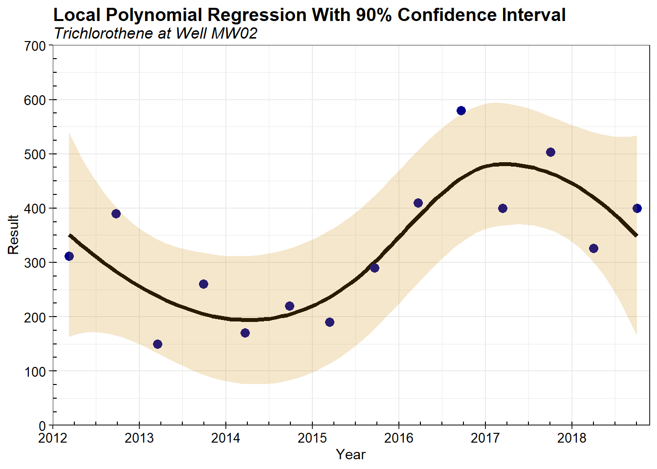
A plot of the local polynomial regression using data for the entire temporal record (base case) is shown below. The shaded region represents the 90% simultaneous confidence interval.
# Create plot
ggplot(data = bpred, aes(x = mesh)) +
  geom_line(aes(y = bpred), size = 1.5) +
  geom_point(data = dat, aes(x = Date, y = Result), color = 'blue4', size = 3) +
  geom_ribbon(aes(ymin = blwr, ymax = bupr), alpha = 0.2, fill = 'orange3') +
  scale_x_continuous(limits = c(2012, 2018.9),
                     breaks = seq(2012, 2018, by = 1),
                     expand = c(0, 0)) +
  scale_y_continuous(limits = c(0, 700),
                     breaks = seq(0, 700, by = 100),
                     expand = c(0, 0),
                     labels = function(x) format(x, big.mark = ",",
                                                 scientific = FALSE)) +
  labs(title = 'Local Polynomial Regression With 90% Confidence Interval',
       subtitle = 'Trichlorothene at Well MW02',
       x = 'Year',
       y = 'Result') +
  theme(plot.title = element_text(margin = margin(b = 2), size = 14,
                                  hjust = 0.0, face = quote(bold)),
        plot.subtitle = element_text(margin = margin(b = 3), size = 12,
                                     hjust = 0.0, face = quote(italic)),
        axis.title.y = element_text(size = 11, color = 'black'),
        axis.title.x = element_text(size = 11, color = 'black'),
        axis.text.x = element_text(size = 10, color = 'black'),
        axis.text.y = element_text(size = 10, color = 'black')) +
  annotation_ticks(sides = 'l', ticks_per_base = 28) +
  annotation_ticks(sides = 'b', ticks_per_base = 28)
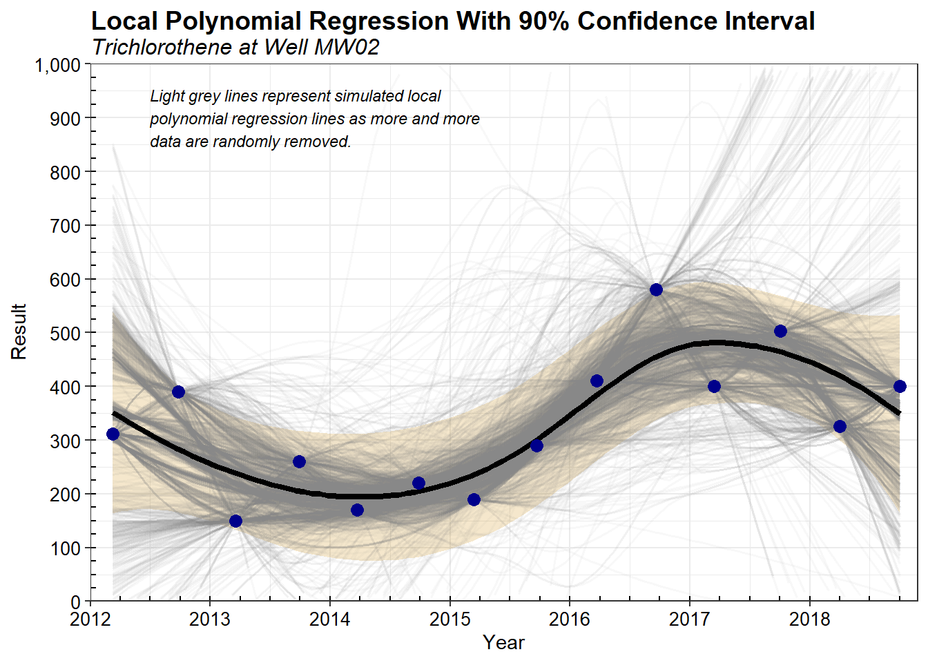
To graphically illustrate the Iterative Thinning process, all the local polynomial regression lines produced during the 200 simulations are shown in the plot below. Each simulation generates multiple lines (in this case, 10), resulting in thousands of regression lines for each well and constituent. Lines that don’t meet the acceptability criterion of having 75% of the line within the 90% confidence interval are not used in the estimation of the final, optimized sampling frequency.
The overall goal in Iterative Thinning is to determine how much data can be removed (and thus how much the interval between sampling events can be lengthened) and still allow reconstruction of the major features of the original trend. Some finer features of the time series trend are undoubtedly lost when less data are collected, but often it is difficult to determine whether these features are real or simply due to measurement and/or field variation in the data. It may also be the case that certain transient features are less important to the needs of the long-term monitoring program and therefore do not need to be estimated as carefully.
# Convert fits to data frame in long format
fits_df <- data.frame(
  matrix(unlist(fits), ncol = length(fits), byrow = FALSE)
  ) %>%
  mutate(mesh = mesh) %>%
  select(mesh, everything()) %>%
  tidyr::gather(sim, result, -mesh)

# Plot with symbols and fit line on top
p <- ggplot(data = bpred, aes(x = mesh)) +
     geom_ribbon(aes(ymin = blwr, ymax = bupr), alpha = 0.2, fill = 'orange3') +
     scale_x_continuous(limits = c(2012, 2018.9),
                        breaks = seq(2012, 2018, by = 1),
                        expand = c(0, 0)) +
     scale_y_continuous(limits = c(0, 1000),
                        breaks = seq(0, 1000, by = 100),
                        expand = c(0, 0),
                        labels = function(x) format(x, big.mark = ",",
                                                    scientific = FALSE)) +
     labs(title = 'Local Polynomial Regression With 90% Confidence Interval',
          subtitle = 'Trichlorothene at Well MW02',
          x = 'Year',
          y = 'Result') +
     theme(plot.title = element_text(margin = margin(b = 2), size = 14,
                                       hjust = 0.0, face = quote(bold)),
           plot.subtitle = element_text(margin = margin(b = 3), size = 12,
                                          hjust = 0.0, face = quote(italic)),
           axis.title.y = element_text(size = 11, color = 'black'),
           axis.title.x = element_text(size = 11, color = 'black'),
           axis.text.x = element_text(size = 10, color = 'black'),
           axis.text.y = element_text(size = 10, color = 'black')) +
     annotation_ticks(sides = 'l', ticks_per_base = 40) +
     annotation_ticks(sides = 'b', ticks_per_base = 28)

# add fits to plot
labell <- paste('Light grey lines represent simulated local',
                'polynomial regression lines as more and more',
                'data are randomly removed.', sep = '\n')
p <- p +
     geom_line(data = fits_df, aes(x = mesh, y = result, group = sim),
       alpha = 0.05, color = 'grey50', size = 0.7) +
     geom_line(data = bpred, aes(x = mesh, y = bpred), color = 'black', size = 1.5) +
     geom_point(data = dat, aes(x = Date, y = Result), color = 'blue4', size = 3) +
     annotate('text', x = 2012.5, y = 900, size = 3, color = 'black', hjust = 0,
              label = labell, fontface = 'italic')
p
Conclusion
The Iterative Thinning routine is data driven, and includes as much useful trend information as is possible. Because local regression is used to estimate non-linear trends in the data at a given well, it does a good job of identifying seasonal patterns that may be present in the data. If a dominant trend cannot be identified in the reduced data, the iterative fitting procedure will register such a result as a loss of accuracy and conclude that too much data has been removed from that well.
While extremely flexible, the Iterative Thinning algorithm has some restrictions. Reliable fitting of an initial trend and confidence intervals around that trend require at least 6 to 10 sample measurements (that is, data from distinct sampling events). Large data gaps in the sampling record may produce artifactual looking trends. The presence of extreme outlying observations in the data also can significantly affect the trend estimate.
References
Cameron, K. 2004. Better Optimization of Long-Term Monitoring Networks. Bioremediation Journal 8:89-107.
Environmental Security Technology Certification Program (ESTCP). 2010. Demonstration and Validation of the Geostatistical Temporal-Spatial Algorithm (GTS) for Optimization of Long-Term Monitoring (LTM) of Groundwater at Military and Government Sites. U.S. Department of Defense ESTCP Cost and Performance Report ER-200714. August.
Loader, C. 1999. Local Regression and Likelihood. Springer, New York.
Pacific Northwest National Laboratory (PNNL). 2014. Visual Sample Plan (VSP) Version 7.0 User’s Guide. Prepared for the U.S. Department of Energy under Contract DE-AC05-76RL01830, Richland, Washington. March.
Science Aplication International Corporation(SAIC). 2004. Final Report Long-Term Monitoring Groundwater Optimzation at Site 49 Pease AFB, New Hampshire Using the Geostatistical Temporal/Spatial (GTS) Algorithm. Submitted to HQ AFCEE/BCE Brooks AFB, Texas. May.
- Posted on:
- March 11, 2021
- Length:
- 13 minute read, 2710 words
- See Also: