Univariate and Multivariate Time-Series Analysis
By Charles Holbert
May 13, 2020
Introduction
Time-series analysis and forecasting is an important area of machine learning because many predictive learning problems involve a time component. Time series analysis and time series forecasting generally have different goals. Time-series analysis is used to describe the components of a time series by decomposing the time series into constitution components, such as seasonal variations, cyclic patterns, long-term trends, and random variations. Assumptions can be made about these components that allow them to be modeled using traditional statistical methods.In contrast, time-series forecasting uses the information in a time series to forecast future values of that series. The components of a time series may be the most effective way to make predictions about future values, but this is not always the case.
An important feature of most time series is that observations close together in time tend to be correlated (serially dependent) and thus, observations are not independent of each other. Most predictive learning methods are based on the assumption that the time series can be rendered approximately stationary (i.e., stationarized) through the use of mathematical transformations. A stationary time series is one whose statistical properties such as the mean, variance, and autocorrelation, are all constant over time. Differences between consecutive observations can be used to achieve stationarity of a non-stationarity dataset. Additionally, log or square-root transformation of the data can be used to stabilize non-constant variance.
To illustrate these concepts, time-series analysis will be performed using indoor air concentrations of trichloroethene (TCE) collected over time at a single location. These time-series data include the following explanatory variables: radon concentration, temperature, barometric pressure, wind direction, wind speed, and working hour. The data will be evaluated to determine the time differencing needed to produce a stationary time series, which will be used to develop univariate and multivariate time series models.
Data
Data quality is an important issue for any project analyzing data. Prior to conducting any statistical analyses, it’s important to analyze the data using various statistical and visualization techniques to bring important aspects of the data into focus for further analysis. For brevity, let’s assume that we have performed a thorough examination of the data.
The data consist of 11 variables with 771 observations averaged over 6-hour internals. The variables include the following:
- Barometric pressure, pascal (BP)
- Date, m/d/yyyy
- Differential temperature (DF)
- Differential pressure (DP)
- Outside temperature, Celsium (Temp)
- Precipitation, inches of water (Precip)
- Radon concentration, picocuries per liter (Radon)
- TCE concentration, micrograms per cubic meter (TCE)
- Wind speed, miles per hour (WS)
- Wind direction (WD)
- Working hour, defined as 6am to 6pm Monday through Friday (WH)
Prior to analysis, barometric pressure was converted from units of Pascal to atmospheres and outside temperature was converted from degrees Celsius to Fahrenheit. Label encoding was used to convert wind direction and working hour to numerical variables. Time entries with missing values for TCE or any of the 10 explanatory variables were removed from the data prior to analysis.
# Load libraries
library(lmtest)
library(forecast)     # Arima, auto.arima, xreg = not a df
library(TSA)          # arima and arimax, xreg = a df
library(tseries)      # Augmented Dickey-Fuller Test
library(rcompanion)   # Tukey Transformation
library(plyr)
library(ggplot2)

# Read data in comma-delimited file
datin <- read.csv(
  './data/NESDI_EIA11data.csv', header = T,
  na.strings = c("", "NA"),
  stringsAsFactors = FALSE
)
datin$Date <- as.POSIXct(datin$Date, format = '%m/%d/%Y %H:%M', tz = 'EST')

# Remove rows having missing values
dat <- na.omit(datin)

# Convert temperature (celcius to F) and pressure (Pa to atm)
dat$Temp <- (9 * dat$Temp / 5 + 32)
dat$BP <- (dat$BP / 101325)

# Assign "ND" to missing wind direction values
dat <- dat %>%
  mutate(WindDir = replace(WindDir, is.na(WindDir), "ND"))

# Create wind direction levels
wind_lvls <- c(
  "N", "NNE", "NE", "ENE", "E",
  "ESE", "SE", "SSE", "S", "SSW",
  "SW", "WSW", "W", "WNW", "NW",
  "NNW", "ND")

# Create ordered factor
dat$WD <- factor(
  dat$WindDir,
   levels = wind_lvls,
  ordered = TRUE
)
dat$WH <- factor(dat$WorkHr, ordered = TRUE)

# Attached the data
attach(dat)
Stationarity
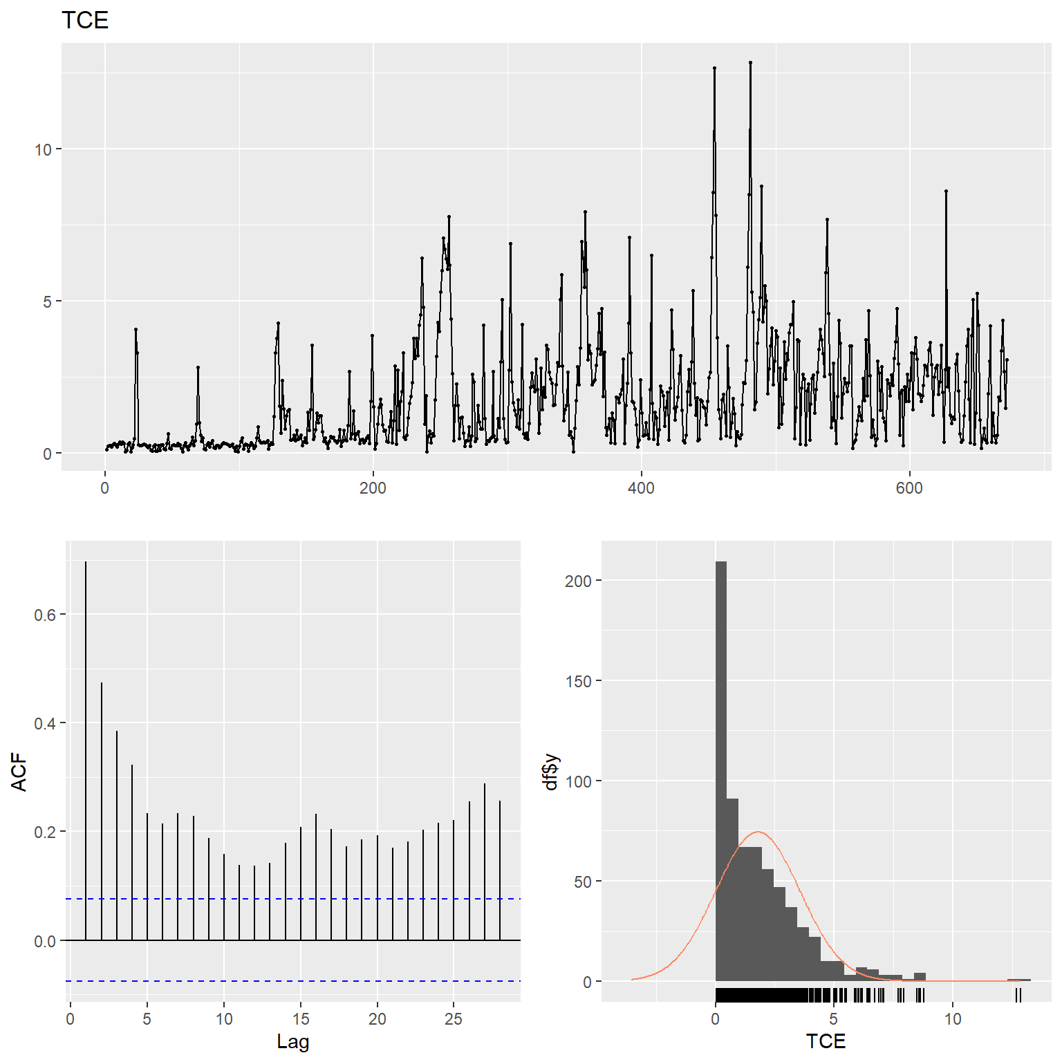
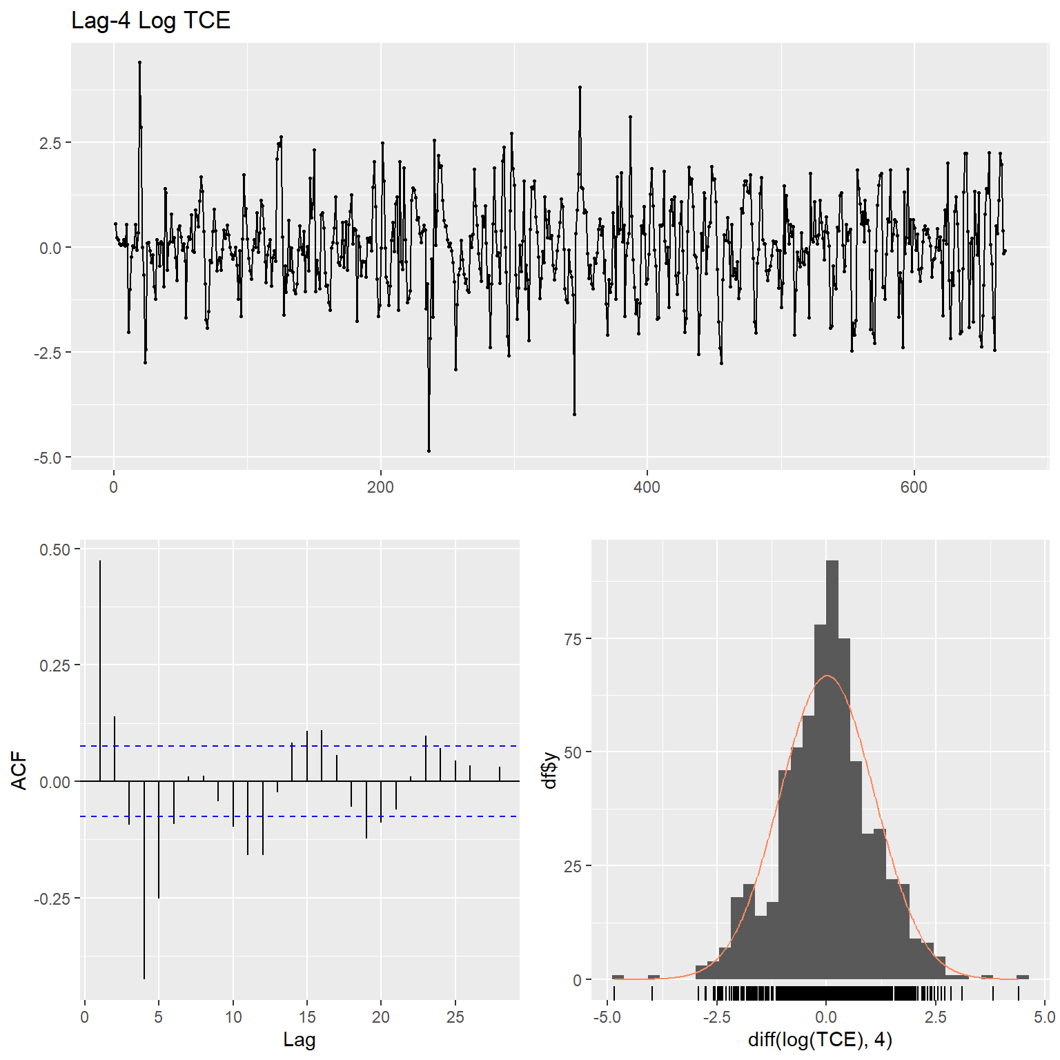
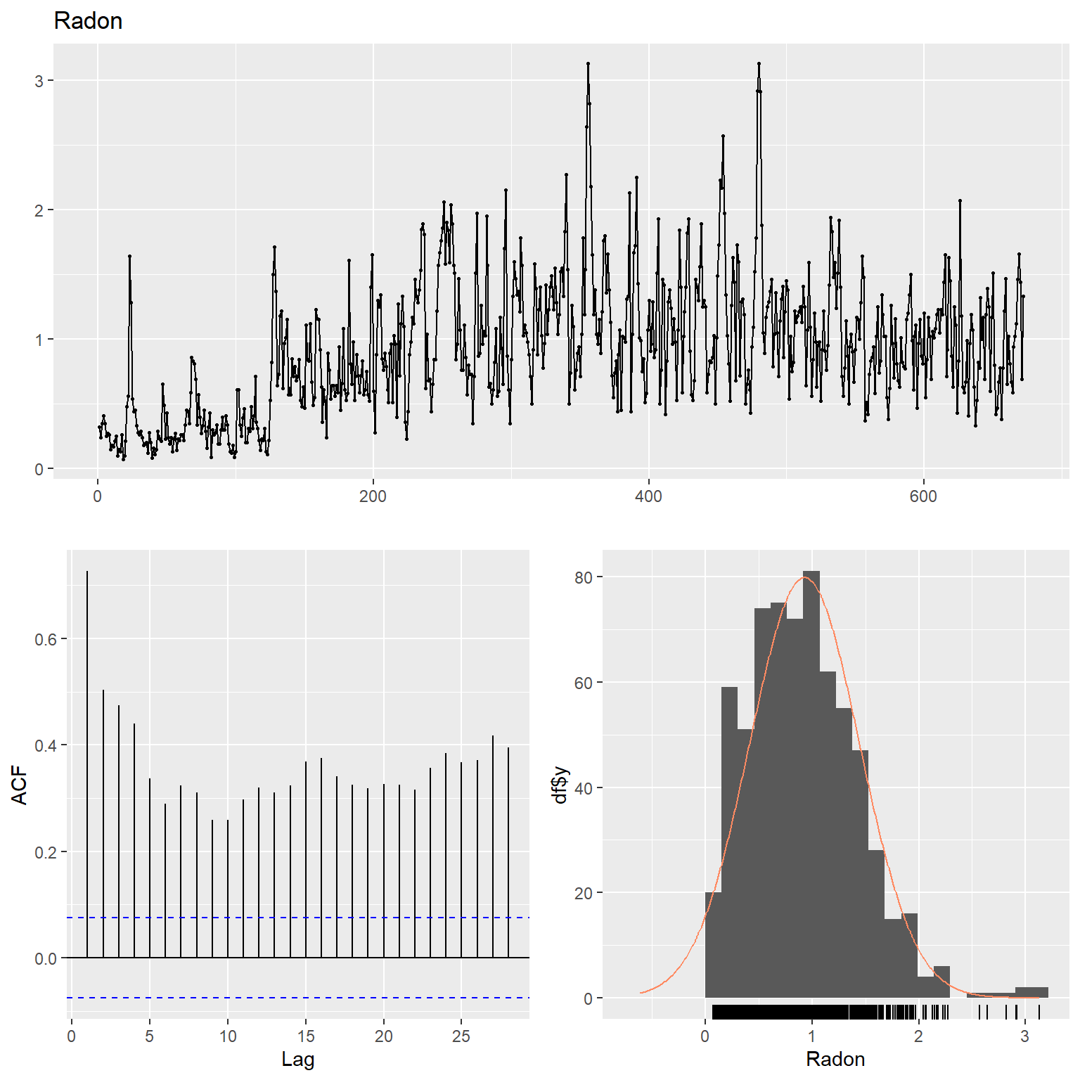
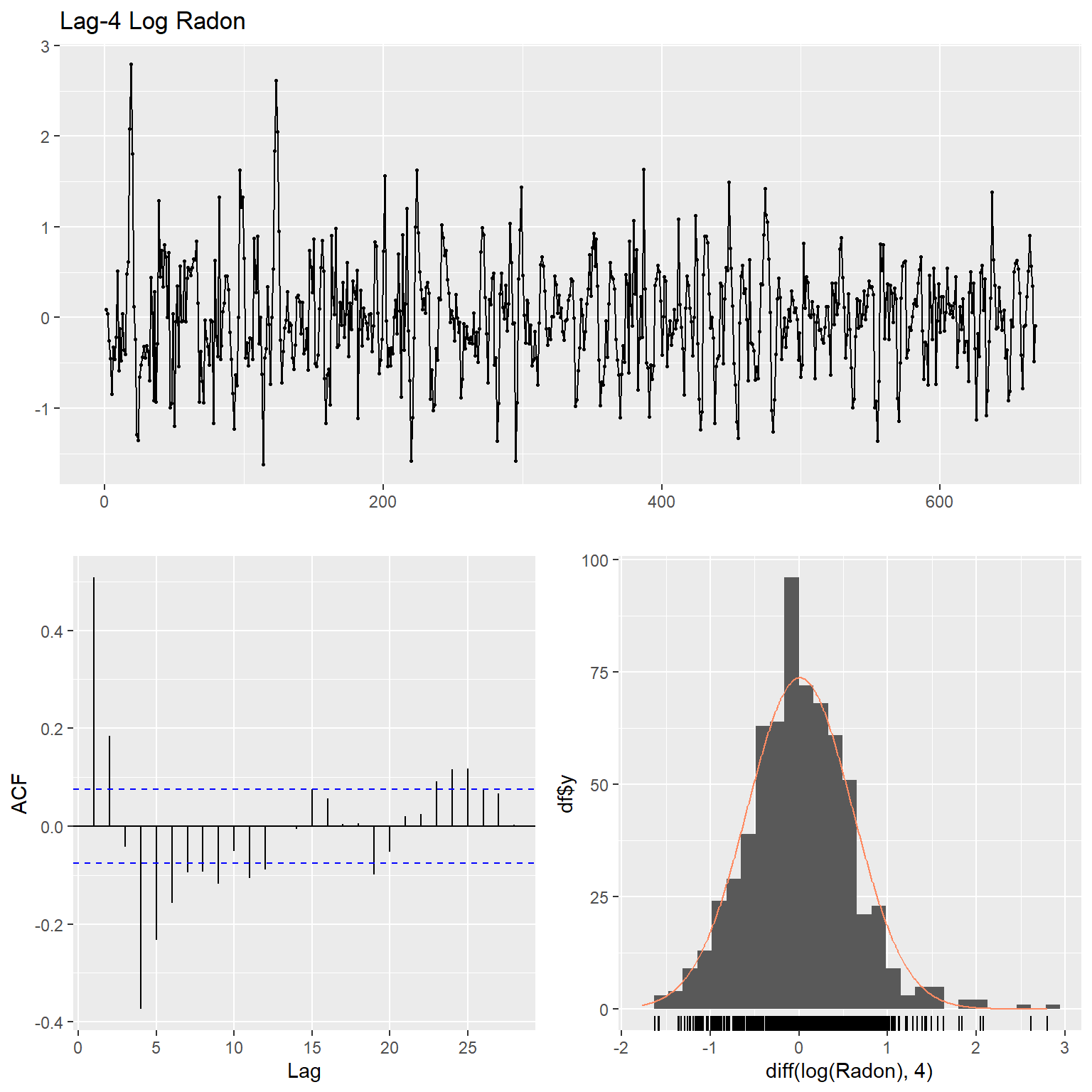
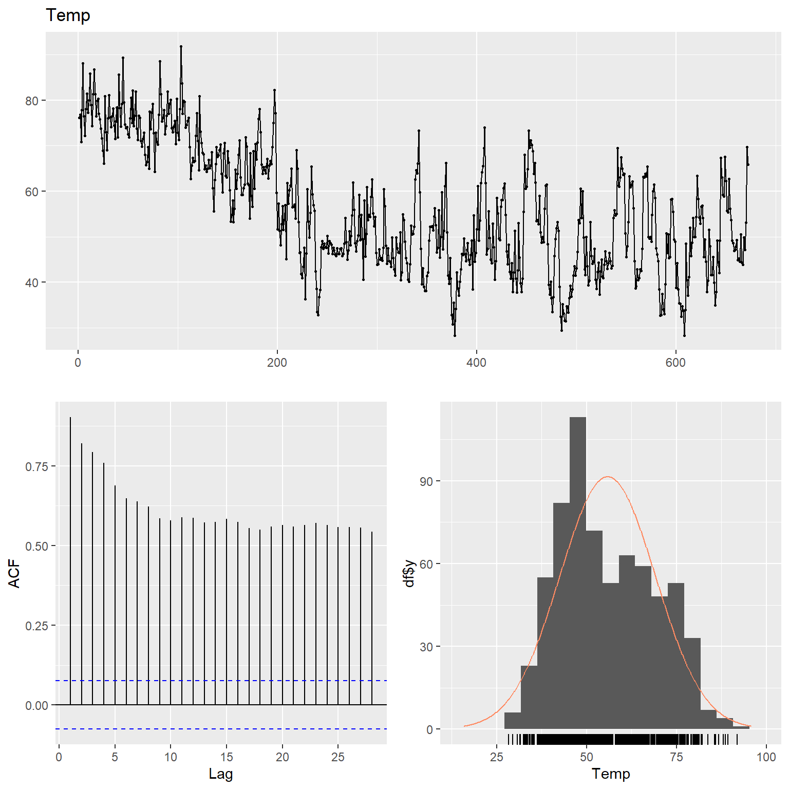
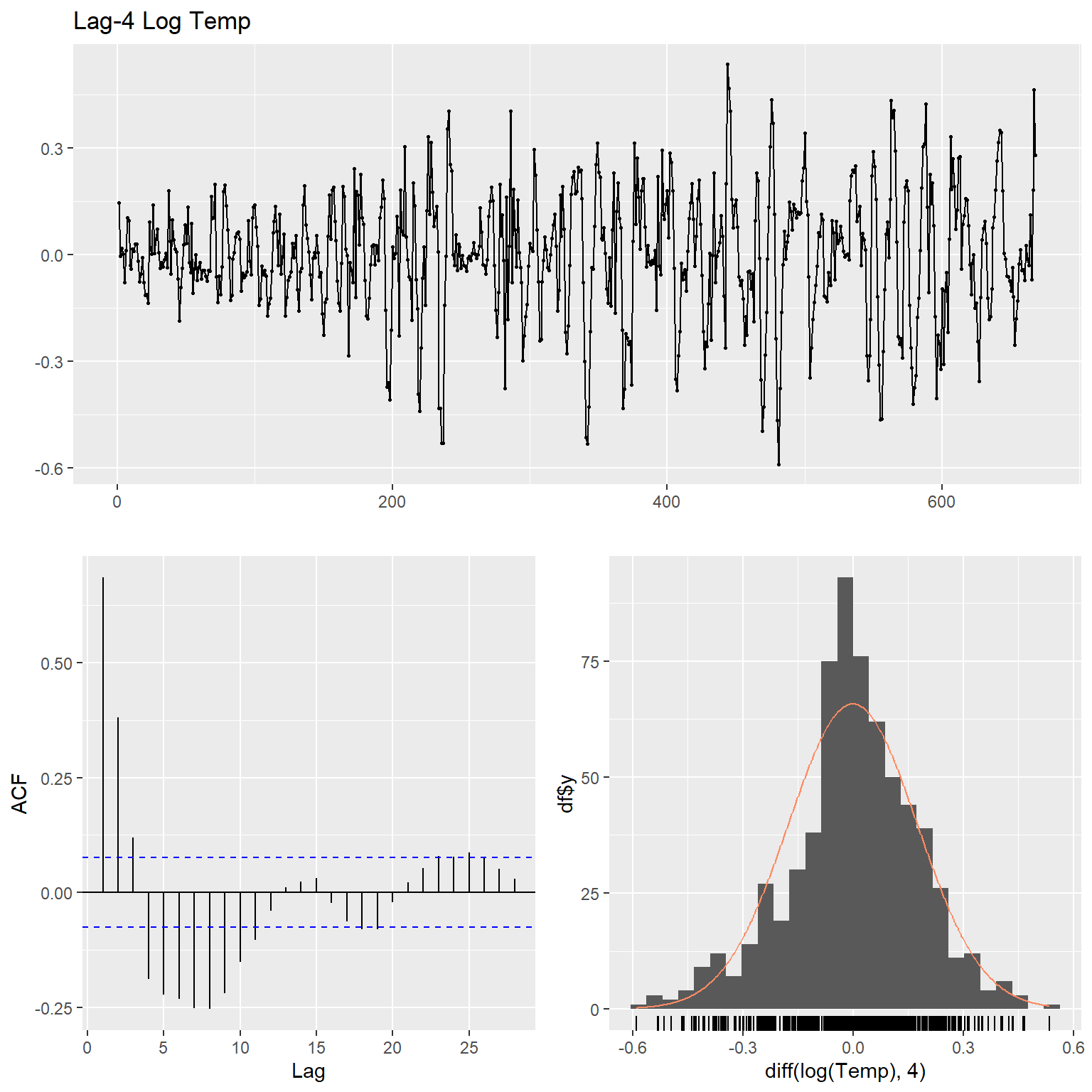
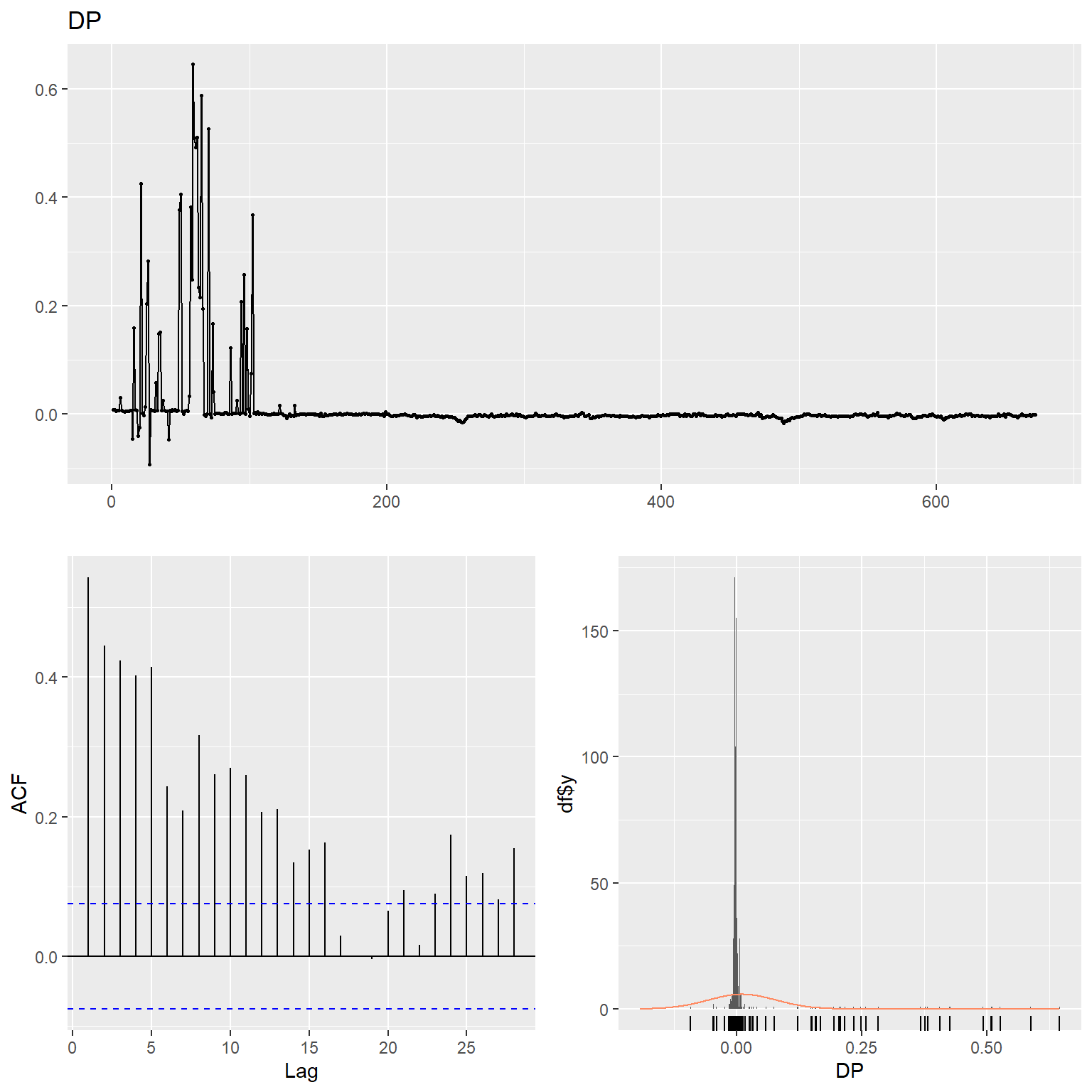
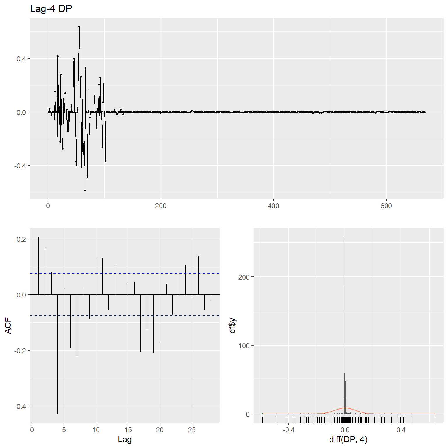
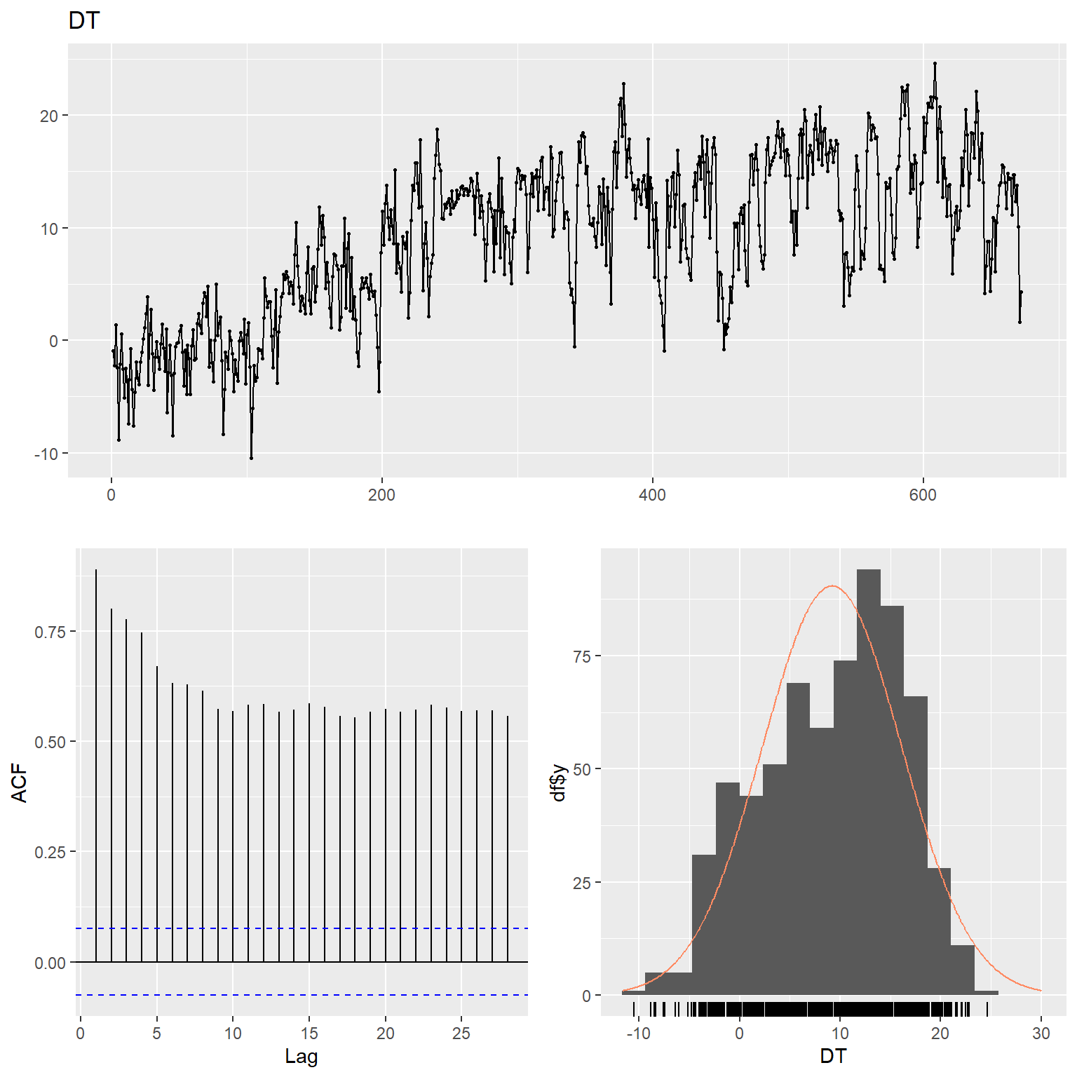
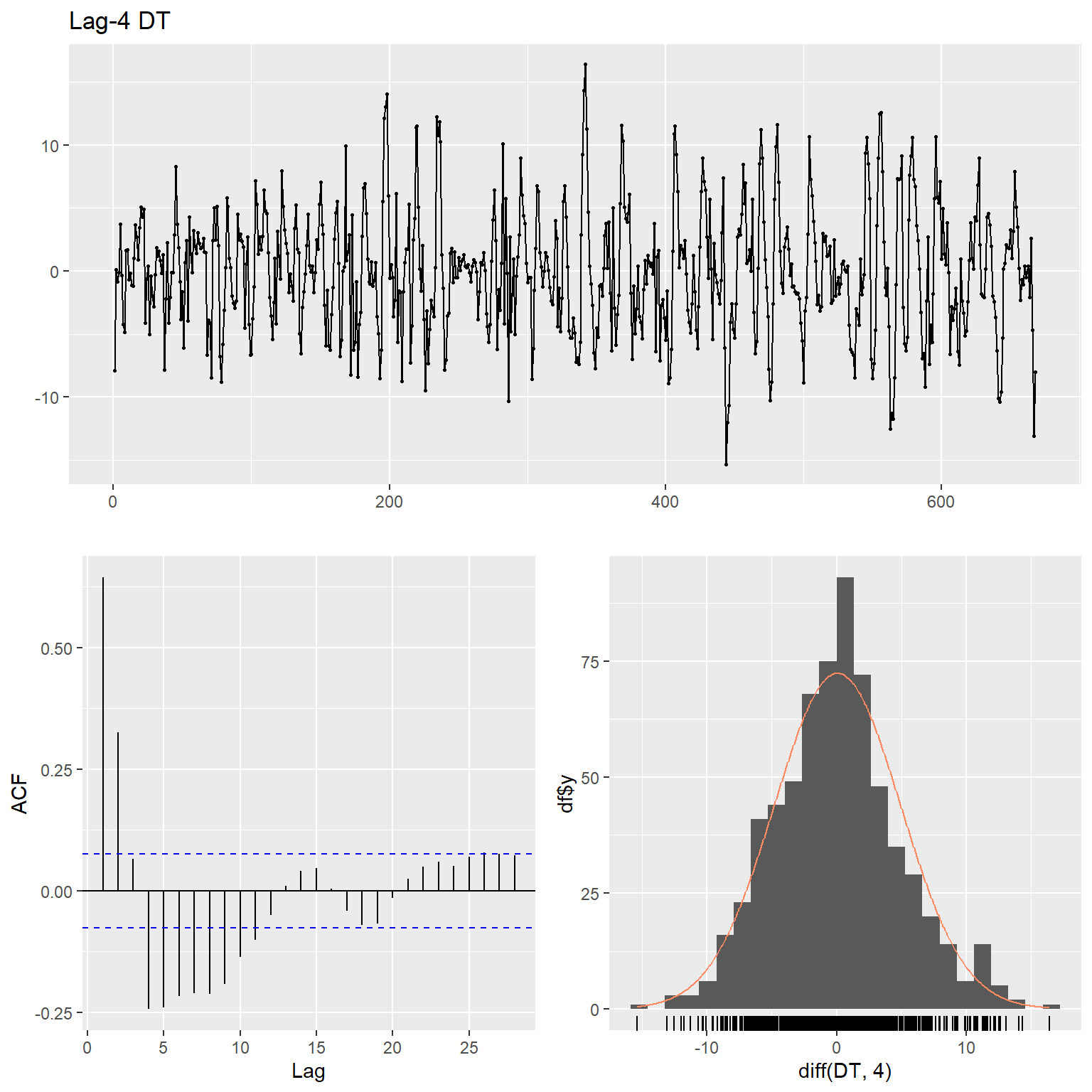
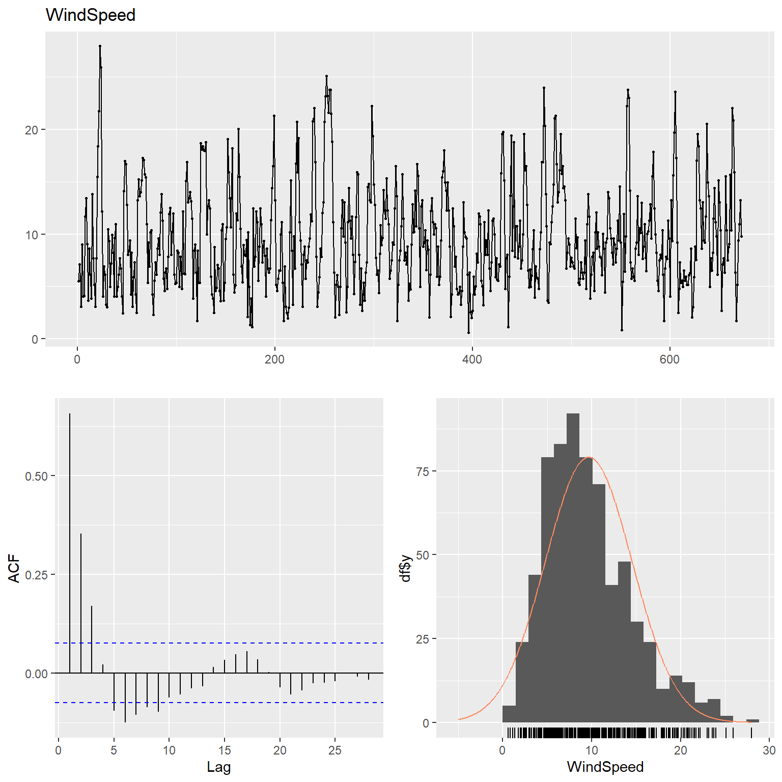
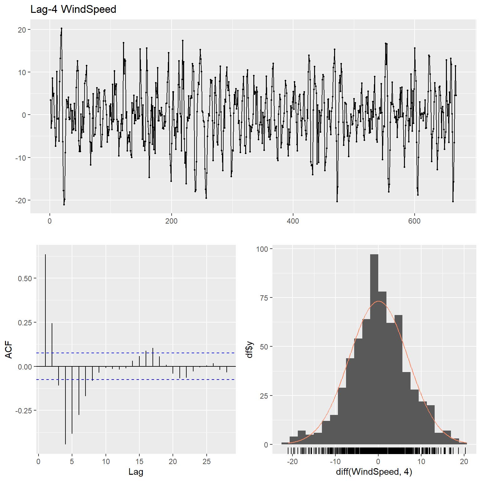
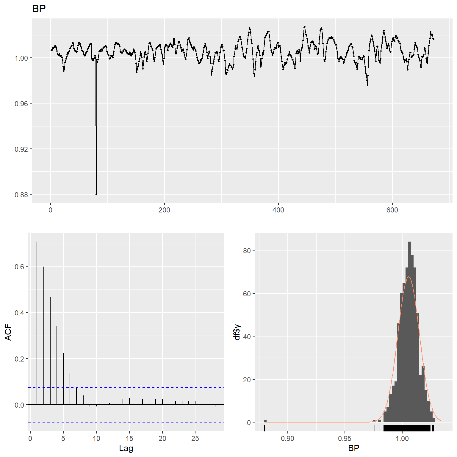
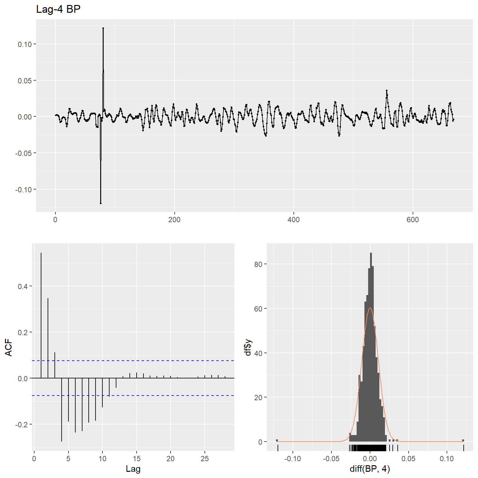
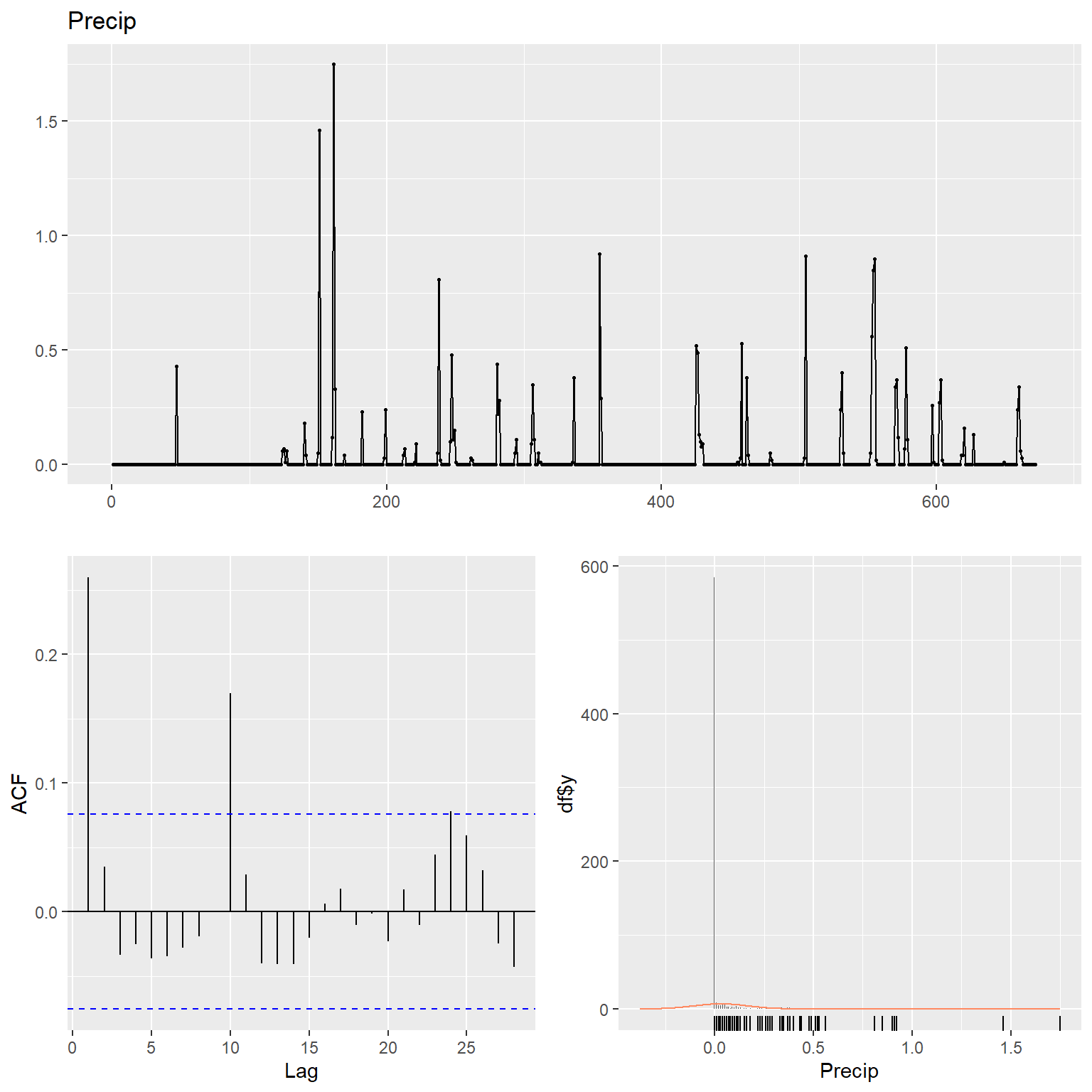
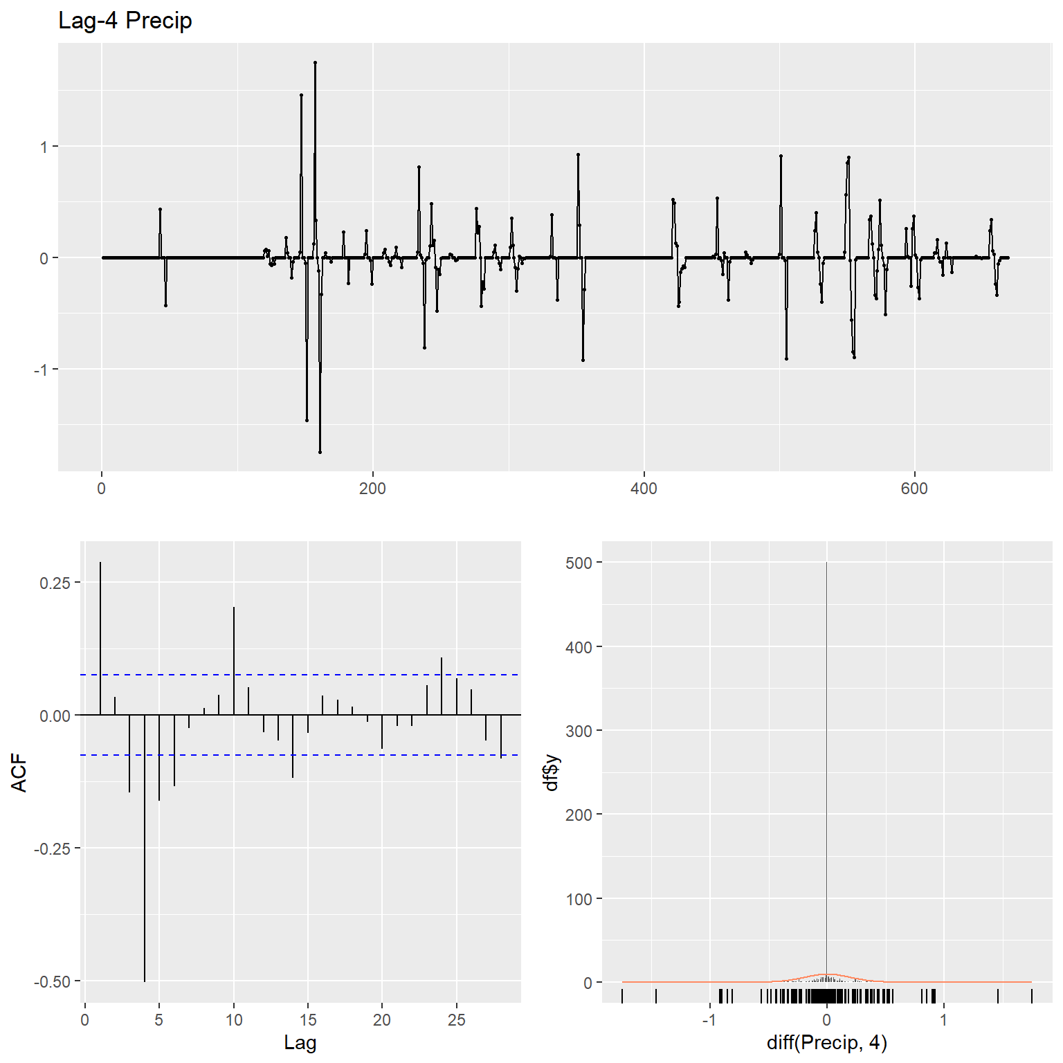
Let’s inspect the data using time series plots, the corresponding autocorrelation function (acf), and the histogram of the raw and lag-4 time differenced data for each variable. The acf gives the autocorrelation at all possible lags. The autocorrelation at lag 0 is included by default which always takes the value 1 as it represents the correlation between the data and themselves. The TCE and radon concentration data exhibit non-constant variance and thus, these data were transformed using natural logarithms to stabilize the variance.
# TCE
ggtsdisplay(
  TCE,
  plot.type = "histogram",
  points = TRUE,
  smooth = FALSE,
  main = "TCE"
)

ggtsdisplay(
  diff(log(TCE), 4),
  plot.type = "histogram",
  points = TRUE,
  smooth = FALSE,
  main = "Lag-4 Log TCE"
)
# Radon
ggtsdisplay(
  Radon,
  plot.type = "histogram",
  points = TRUE,
  smooth = FALSE,
  main = "Radon"
)

ggtsdisplay(
  diff(log(Radon), 4),
  plot.type = "histogram",
  points = TRUE,
  smooth = FALSE,
  main = "Lag-4 Log Radon"
)
# Temp
ggtsdisplay(
  Temp,
  plot.type = "histogram",
  points = TRUE,
  smooth = FALSE,
  main = "Temp"
)

ggtsdisplay(
  diff(log(Temp), 4),
  plot.type = "histogram",
  points = TRUE,
  smooth = FALSE,
  main = "Lag-4 Log Temp"
)
# DP
ggtsdisplay(
  DP,
  plot.type = "histogram",
  points = TRUE,
  smooth = FALSE,
  main = "DP"
)

ggtsdisplay(
  diff(DP, 4),
  plot.type = "histogram",
  points = TRUE,
  smooth = FALSE,
  main = "Lag-4 DP"
)
# DT
ggtsdisplay(
  DT,
  plot.type = "histogram",
  points = TRUE,
  smooth = FALSE,
  main = "DT"
)

ggtsdisplay(
  diff(DT, 4),
  plot.type = "histogram",
  points = TRUE,
  smooth = FALSE,
  main = "Lag-4 DT"
)
# WindSpeed
ggtsdisplay(
  WindSpeed,
  plot.type = "histogram",
  points = TRUE,
  smooth = FALSE,
  main = "WindSpeed"
)

ggtsdisplay(
  diff(WindSpeed, 4),
  plot.type = "histogram",
  points = TRUE,
  smooth = FALSE,
  main = "Lag-4 WindSpeed"
)
# BP
ggtsdisplay(
  BP,
  plot.type = "histogram",
  points = TRUE,
  smooth = FALSE,
  main = "BP"
)

ggtsdisplay(
  diff(BP, 4),
  plot.type = "histogram",
  points = TRUE,
  smooth = FALSE,
  main = "Lag-4 BP"
)
# Precip
ggtsdisplay(
  Precip,
  plot.type = "histogram",
  points = TRUE,
  smooth = FALSE,
  main = "Precip"
)

ggtsdisplay(
  diff(Precip, 4),
  plot.type = "histogram",
  points = TRUE,
  smooth = FALSE,
  main = "Lag-4 Precip"
)
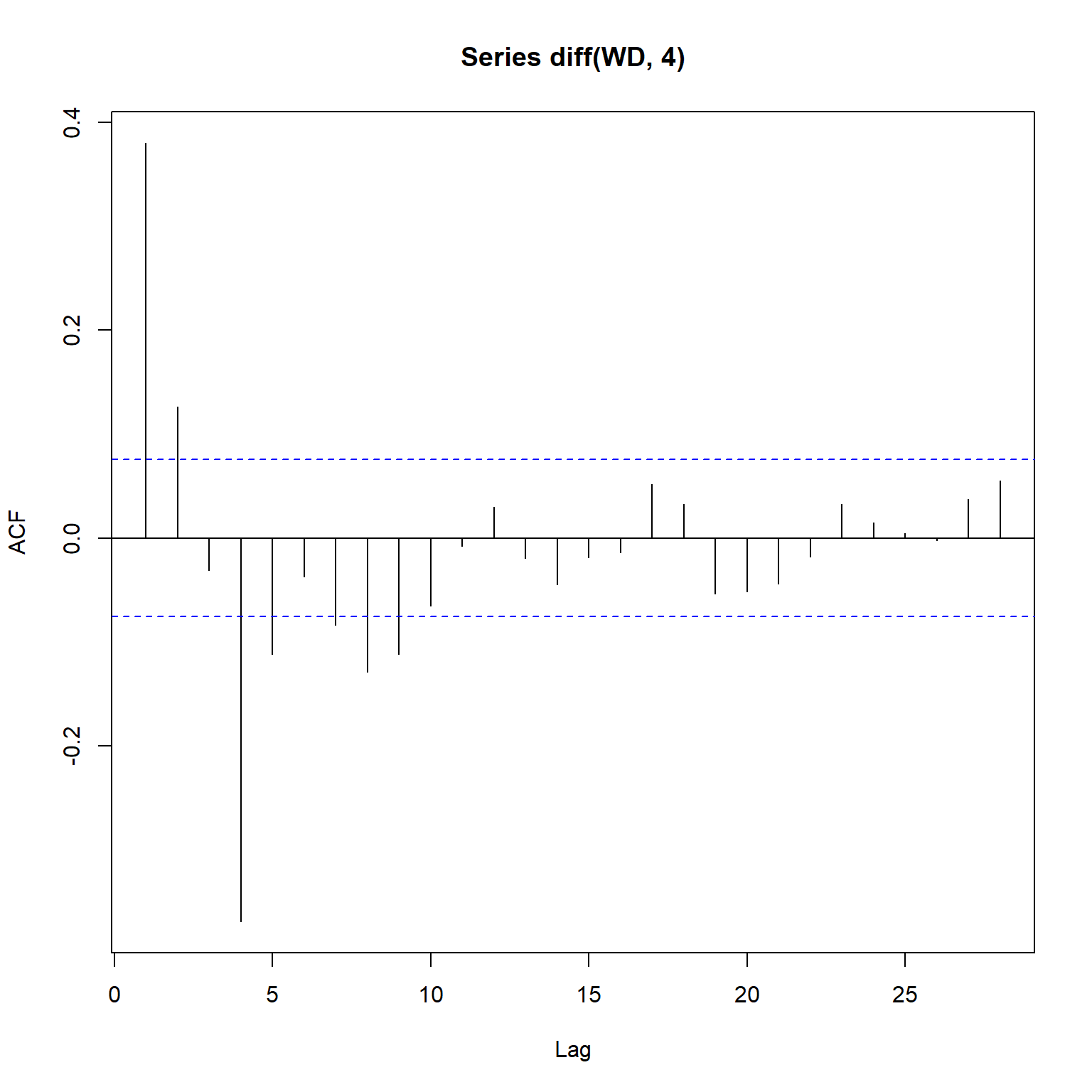
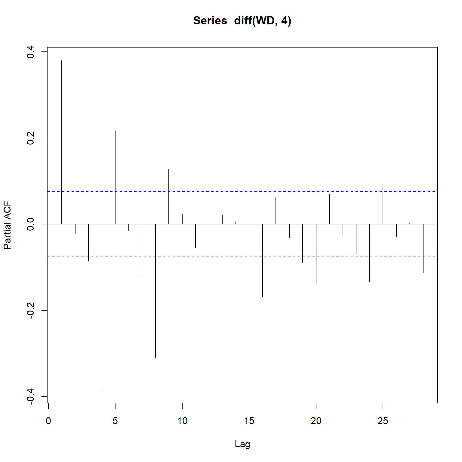
Working hours (WH) only has two categories so let’s inspect the acf and the partial autocorrelation function (pacf). The pacf is a summary of the relationship between an observation in a time series with observations at prior time steps with the relationships of intervening observations removed. It contrasts with the autocorrelation function, which does not control for other lags.
# WD
acf(diff(WD, 4))
pacf(diff(WD, 4))
yts <- ts(log(TCE))
x1ts <- ts(log(Radon))
x2ts <- ts(DP)
x3ts <- ts(DT)
x4ts <- ts(Temp)
x5ts <- ts(WindSpeed)
x6ts <- ts(BP)
x7ts <- ts(Precip)
x8ts <- ts(WH)
x9ts <- ts(WD)
After creating time series of the lag-4 time differenced, log-transformed TCE data, let’s test the data for stationarity using the augmented Dickey-Fuller (ADF) test (Fuller 1996). The ADF test is a common statistical test used to test whether a given time series is stationary or not. The ADF method tests for unit root stationary with a null hypothesis that the data are non-stationary. In general, a stationary time series should have no predictable patterns (i.e., no trend or seasonality). Therefore when we run the test, low p-values indicate stationarity.
TCE <- window(yts, end = 538)
adf.test(diff(TCE, 4))
##
## 	Augmented Dickey-Fuller Test
##
## data:  diff(TCE, 4)
## Dickey-Fuller = -9.9986, Lag order = 8, p-value = 0.01
## alternative hypothesis: stationary
The p-value is 0.01, so we can reject the null hypothesis of non-stationarity at the 5 percent significance level. This means that lag-4 time differenced, log-transformed TCE data satisfies the stationarity requirement of time series modeling. Now, let’s test the lag-4 time differenced, log-transformed radon data.
Radon <- x1ts
adf.test(diff(Radon,4))
##
## 	Augmented Dickey-Fuller Test
##
## data:  diff(Radon, 4)
## Dickey-Fuller = -11.452, Lag order = 8, p-value = 0.01
## alternative hypothesis: stationary
The p-value is less than the 5 percent significance level and hence we can reject the null hypothesis of non-stationarity and assume that the radon series is stationary.
Time Series Modelling
Time series data analysis means analyzing the available data to identify the pattern or trend in the data, generally to predict some future values. A widely used statistical method for time series analysis is the Auto-Regressive Integrated Moving Average (ARIMA) model (Hyndman and Athanasopoulos 2013). This class of model explains a given time series based on its own past values, that is, its own lags and the lagged forecast errors. ARIMA models are typically expressed as ARIMA(p,d,q), with the three terms p, d, and q defined as follows:
- p - number of lag observations included in the autoregression model (lag order)
- d - number of times that the raw observations are differenced (degree of differencing).
- q - size of the moving average window (order of moving average).
Univariate Time Series Model for TCE
First, let’s fit the best univariate ARIMA model to the lag-4 time differenced, log-transformed TCE data. A univariate time series model includes the variable to be modelled and the corresponding date/time for each observation. The data will be split into a training and test (or holdout) set. The training set, consisting of 80% of the complete data, will be used to fit the model. The test set, consisting of 20% of the complete data, will be used to evaluate the performance of the selected model on unseen data.
yfit <- arima(
  TCE, order = c(1, 0, 2),
  seasonal = list(order = c(0, 1, 1), period = 4)
)
yfit
##
## Call:
## arima(x = TCE, order = c(1, 0, 2), seasonal = list(order = c(0, 1, 1), period = 4))
##
## Coefficients:
##          ar1      ma1      ma2     sma1
##       0.8028  -0.2175  -0.1892  -0.9217
## s.e.  0.0661   0.0791   0.0593   0.0205
##
## sigma^2 estimated as 0.5239:  log likelihood = -588.76,  aic = 1185.52
Let’s inspect the coefficients for this model.
coeftest(yfit)
##
## z test of coefficients:
##
##       Estimate Std. Error  z value  Pr(>|z|)
## ar1   0.802761   0.066082  12.1480 < 2.2e-16 ***
## ma1  -0.217471   0.079068  -2.7504  0.005952 **
## ma2  -0.189152   0.059280  -3.1908  0.001419 **
## sma1 -0.921652   0.020510 -44.9358 < 2.2e-16 ***
## ---
## Signif. codes:  0 '***' 0.001 '**' 0.01 '*' 0.05 '.' 0.1 ' ' 1
It appears the best univariate model for TCE is ARIMA(1,0,2)(0,1,1). Both the stationarity and invertibility constraints are satisfied by the estimated coefficients. Invertibility implies that we can express the errors as the weighted sum of current and prior observations.
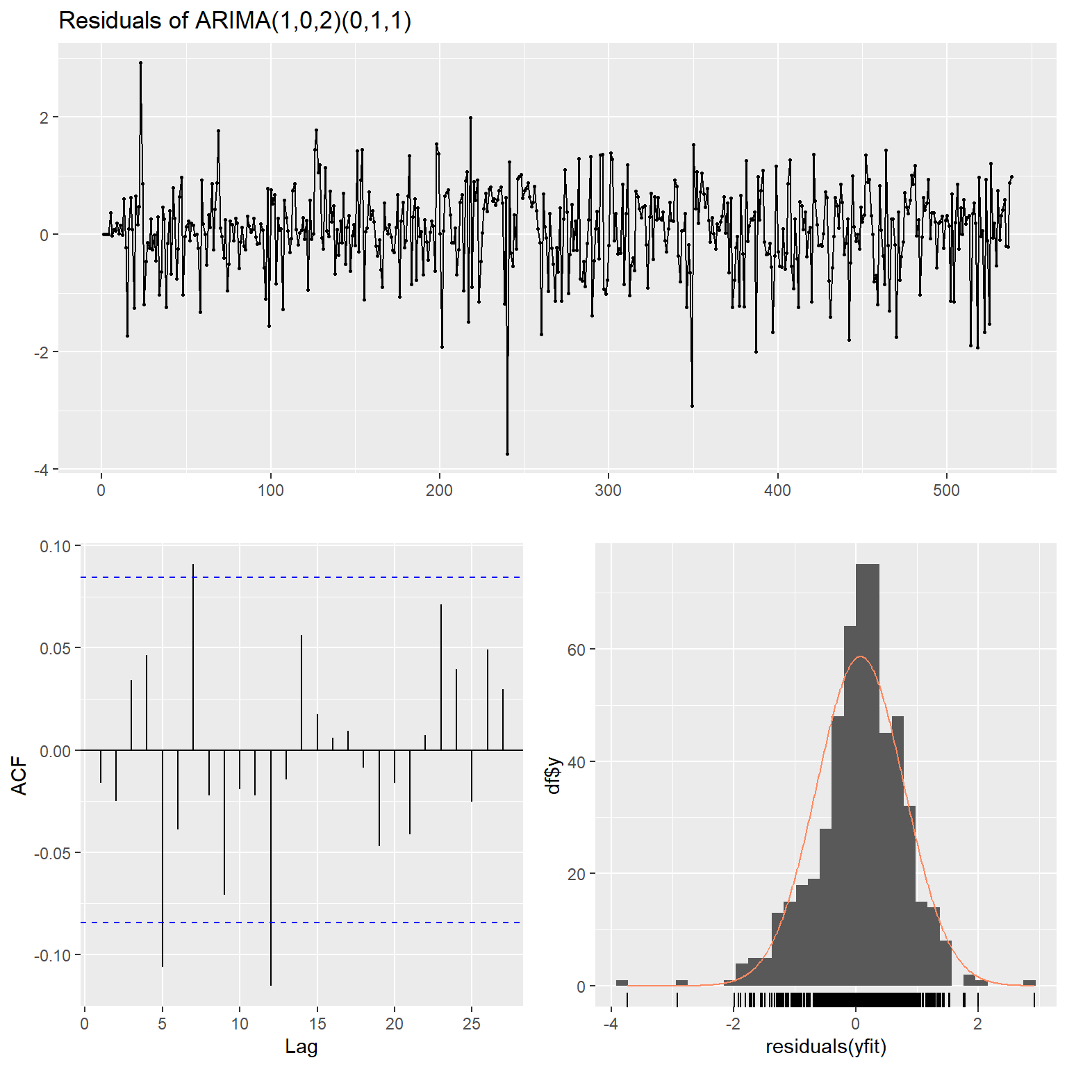
Let’s inspect the residual characteristics for this model. The residual error plots (e.g., scatter, autocorrelation, and histogram plots) indicate no evidence of any systematic autocorrlation in the residual errors of the fitted model. There are, however, a few statistically significant autocorrelations at lags 5, 7, and 12. Practically speaking, it doesn’t appear to be reasonable to further accomodate these higher lag, unsystematic autocorrelations in the model.
ggtsdisplay(
  residuals(yfit),
  plot.type = "histogram",
  points = TRUE,
  smooth = FALSE,
  main = "Residuals of ARIMA(1,0,2)(0,1,1)"
)
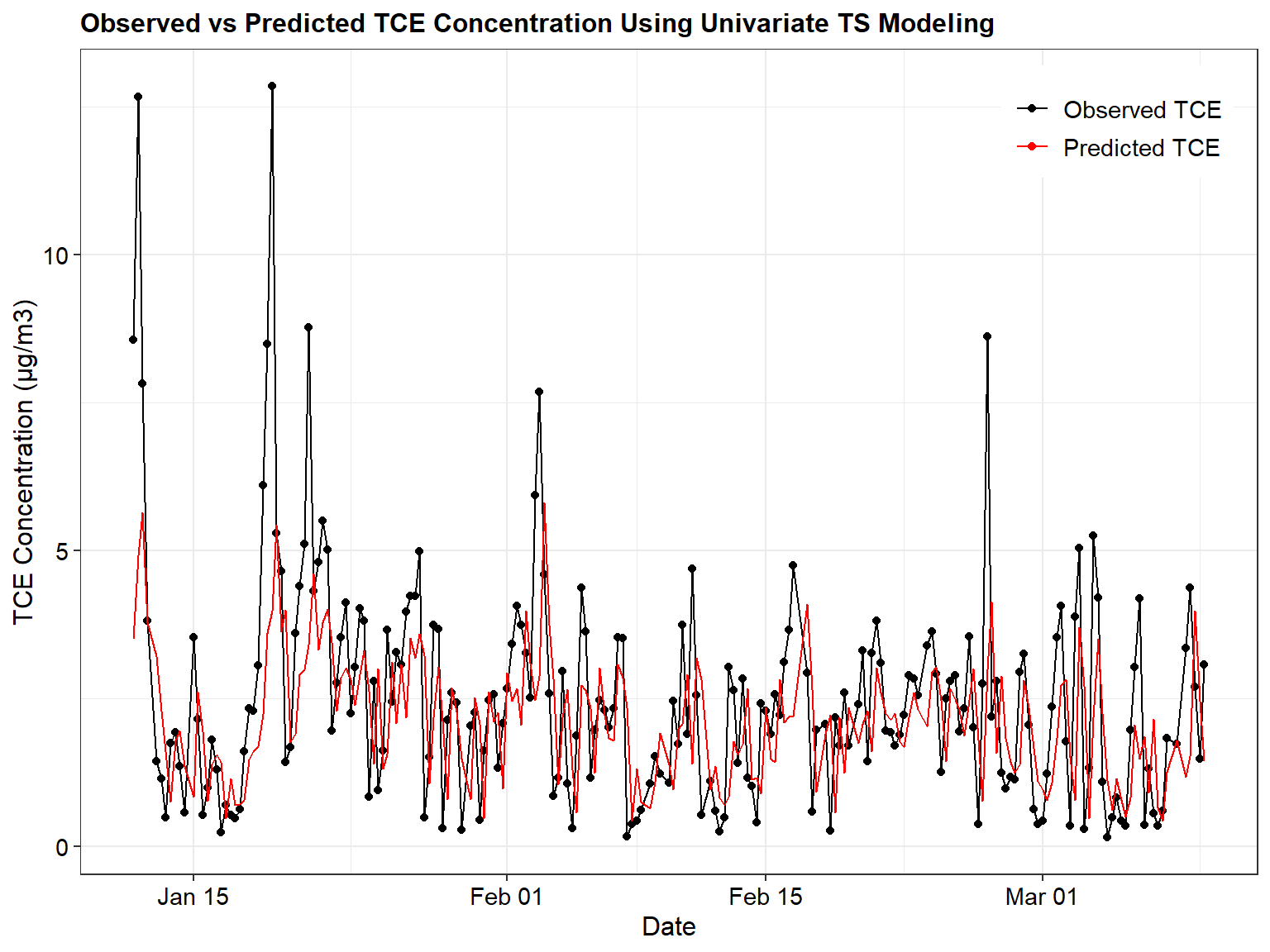
Let’s see how the predicted values for this model compare to the actual observations.
# Comparison of observed results to predicted results
newfit1 <- Arima(yts, model = yfit)
dat$Arima_Predicted <- fitted(newfit1)

ggplot(data = subset(dat, ObsNumber >= 539),
       aes(x = Date)) +
  geom_point(aes(y = TCE, color = "Observed TCE"))+
  geom_line(aes(y = TCE, color = "Observed TCE")) +
  geom_line(aes(y = exp(Arima_Predicted), color = "Predicted TCE")) +
  labs(title = "Observed vs Predicted TCE Concentration Using Univariate TS Modeling",
       x = "Date",
       y = "TCE Concentration (µg/m3)") +
  scale_color_manual(breaks = c("Observed TCE",
                                "Predicted TCE"),
                     values = c("Observed TCE" = "black",
                                "Predicted TCE" = "red")) +
  theme_bw() +
  theme(plot.title = element_text(size = 12, hjust = 0, color = 'black', face = quote(bold)),
        axis.title.y = element_text(size = 12, color = 'black'),
        axis.title.x = element_text(size = 12, color = 'black'),
        axis.text.x = element_text(size = 11, color = 'black'),
        axis.text.y = element_text(size = 11, color = 'black'),
        legend.position = c(0.98, 0.98),
        legend.justification = c(1, 1),
        legend.title = element_blank(),
        legend.text = element_text(size = 11))
Univariate Time Series Model for Radon
Similar to the time series model for TCE, one can fit a univariate time series ARIMA model to the lag-4 time differenced, log-transformed radon data.
x1fit <- Arima(Radon, order = c(2,0,1),
               seasonal = list(order = c(1, 1, 1), period = 4))
x1fit
## Series: Radon
## ARIMA(2,0,1)(1,1,1)[4]
##
## Coefficients:
##           ar1     ar2     ma1    sar1     sma1
##       -0.1704  0.3505  0.8153  0.1343  -0.8900
## s.e.   0.0906  0.0664  0.0755  0.0486   0.0225
##
## sigma^2 = 0.1557:  log likelihood = -327.22
## AIC=666.44   AICc=666.57   BIC=693.47
Let’s inspect the coefficients for the Radon model.
coeftest(x1fit)
##
## z test of coefficients:
##
##       Estimate Std. Error  z value  Pr(>|z|)
## ar1  -0.170433   0.090588  -1.8814  0.059916 .
## ar2   0.350483   0.066367   5.2809 1.285e-07 ***
## ma1   0.815314   0.075520  10.7961 < 2.2e-16 ***
## sar1  0.134316   0.048590   2.7643  0.005705 **
## sma1 -0.890019   0.022531 -39.5027 < 2.2e-16 ***
## ---
## Signif. codes:  0 '***' 0.001 '**' 0.01 '*' 0.05 '.' 0.1 ' ' 1
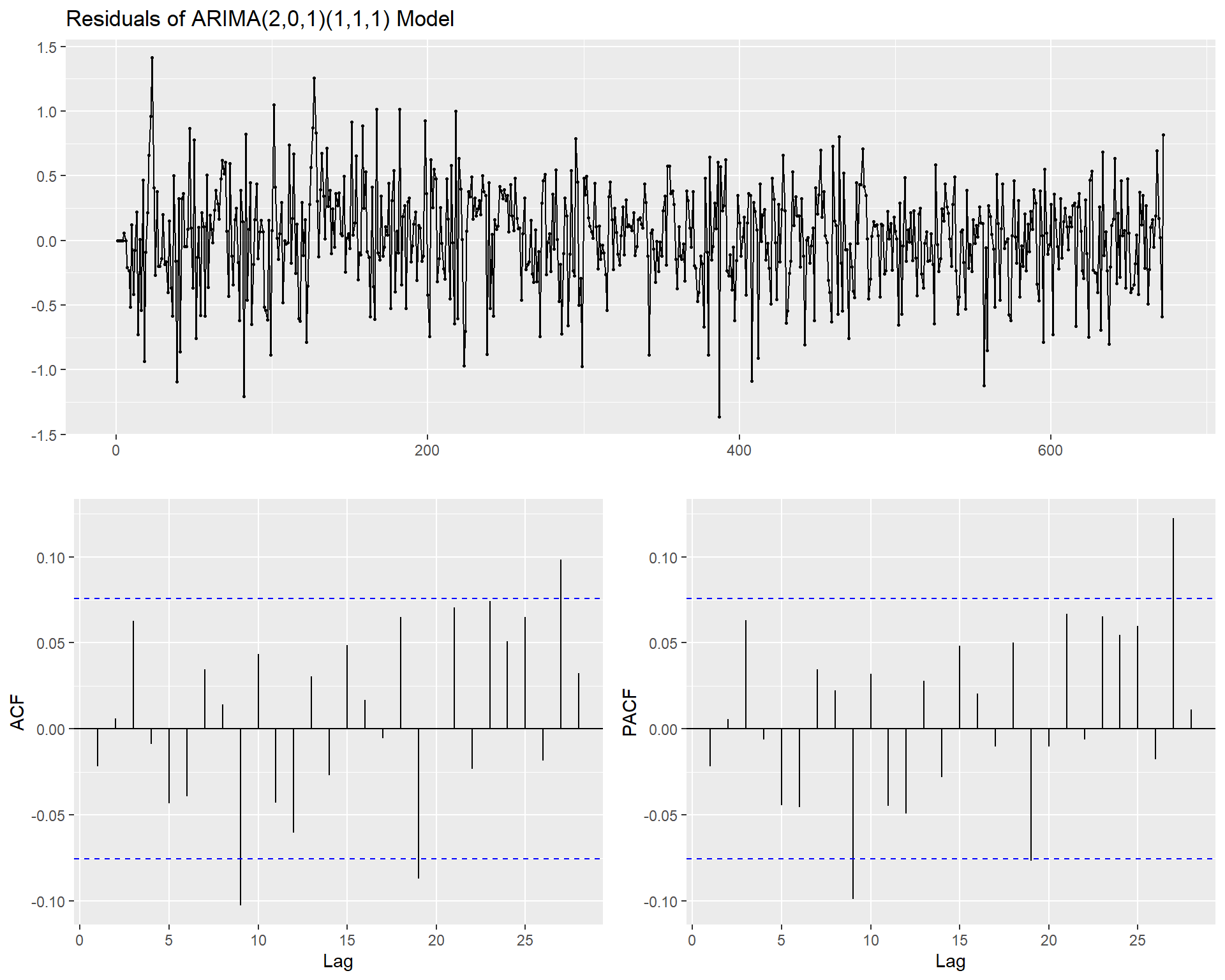
Let’s inspect the residual characteristics for the radon model.
ggtsdisplay(
  residuals(x1fit),
  plot.type = "partial",
  points = TRUE,
  smooth = FALSE,
  main = "Residuals of ARIMA(2,0,1)(1,1,1) Model"
)
Multivariate Time Series Model for TCE
Model 1
Let’s develop a regression time series model with autocorrelated errors for TCE using a low-order proxy ARIMA. To develop a multivariate time series model, data having a sufficiently large number of lags are used so that the model captures the longest time-lagged response that is likely to be important. All explanatory variables will be used in this first model.
#Creat lagged data set
xy.ts <- ts.intersect(
  yts,
  x1ts, lag(x1ts, -1), lag(x1ts, -2), lag(x1ts, -3), lag(x1ts, -4),
  lag(x1ts, -5), lag(x1ts, -6), lag(x1ts, -7), lag(x1ts, -8),
  lag(x1ts, -9), lag(x1ts, -10), lag(x1ts, -11), lag(x1ts, -12),
  x2ts, lag(x2ts, -1), lag(x2ts, -2), lag(x2ts, -3), lag(x2ts, -4),
  lag(x2ts, -5), lag(x2ts, -6), lag(x2ts, -7), lag(x2ts, -8),
  lag(x2ts, -9), lag(x2ts, -10), lag(x2ts, -11), lag(x2ts, -12),
  x3ts, lag(x3ts, -1), lag(x3ts, -2), lag(x3ts, -3), lag(x3ts, -4),
  lag(x3ts, -5), lag(x3ts, -6), lag(x3ts, -7), lag(x3ts, -8),
  lag(x3ts, -9), lag(x3ts, -10), lag(x3ts, -11), lag(x3ts, -12),
  x4ts, lag(x4ts, -1), lag(x4ts, -2), lag(x4ts, -3), lag(x4ts, -4),
  x5ts, lag(x5ts, -1), lag(x5ts, -2), lag(x5ts, -3), lag(x5ts, -4),
  x6ts, lag(x6ts, -1), lag(x6ts, -2), lag(x6ts, -3), lag(x6ts, -4),
  x7ts, lag(x7ts, -1), lag(x7ts, -2), lag(x7ts, -3), lag(x7ts, -4),
  x8ts, lag(x8ts, -1), lag(x8ts, -2), lag(x8ts, -3), lag(x8ts, -4),
  x9ts, lag(x9ts, -1), lag(x9ts, -2), lag(x9ts, -3), lag(x9ts, -4)
)
y.data <- xy.ts[,1]
x.data <- cbind(
  radon0 = xy.ts[,2], radon1 = xy.ts[,3], radon2 = xy.ts[,4],
  radon3 = xy.ts[,5], radon4 = xy.ts[,6], radon5 = xy.ts[,7], radon6 = xy.ts[,8],
  radon7 = xy.ts[,9], radon8 = xy.ts[,10], radon9 = xy.ts[,11], radon10 = xy.ts[,12],
  DP0 = xy.ts[,13], DP1 = xy.ts[,14], DP2 = xy.ts[,15], DP3 = xy.ts[,16],
  DP4 = xy.ts[,17], DP5 = xy.ts[,18], DP6 = xy.ts[,19], DP7 = xy.ts[,20],
  DP8 = xy.ts[,21], DP9 = xy.ts[,22], DP10 = xy.ts[,23],
  DT0 = xy.ts[,24], DT1 = xy.ts[,25], DT2 = xy.ts[,26], DT3 = xy.ts[,27],
  DT4 = xy.ts[,28], DT5 = xy.ts[,29], DT6 = xy.ts[,30], DT7 = xy.ts[,31],
  DT8 = xy.ts[,32], DT9 = xy.ts[,33], DT10 = xy.ts[,34],
  TEMP0 = xy.ts[,35], TEMP1 = xy.ts[,36], TEMP2 = xy.ts[,37], TEMP3 = xy.ts[,38],
  WindSpeed0 = xy.ts[,39], WindSpeed1 = xy.ts[,40], WindSpeed2 = xy.ts[,41],
  WindSpeed3 = xy.ts[,42], BP0 = xy.ts[,43], BP1 = xy.ts[,44], BP2 = xy.ts[,45],
  BP3 = xy.ts[,46], Precip0 = xy.ts[,47], Precip1 = xy.ts[,48], Precip2 = xy.ts[,49],
  Precip3 = xy.ts[,50], WH0 = xy.ts[,51], WH1 = xy.ts[,52], WH2 = xy.ts[,53],
  WH3 = xy.ts[,54], WD0 = xy.ts[,55], WD1 = xy.ts[,56], WD2 = xy.ts[,57],
  WD3 = xy.ts[,58]
)
mod1 <- Arima(window(y.data, end = 538),
              xreg = window(x.data, end = 538),
              order = c(1, 0, 0),
              seasonal = list(order = c(0, 1, 0), period = 4))
mod1
## Series: window(y.data, end = 538)
## Regression with ARIMA(1,0,0)(0,1,0)[4] errors
##
## Coefficients:
##          ar1  radon0  radon1  radon2   radon3   radon4   radon5   radon6
##       0.2397  1.2259  0.1070  0.1257  -0.0699  -0.0058  -0.1265  -0.0118
## s.e.  0.0434  0.0688  0.0729  0.0725   0.0712   0.0848   0.0801   0.0792
##       radon7   radon8  radon9  radon10     DP0      DP1      DP2      DP3
##       0.1644  -0.0326  0.0319  -0.0726  0.0295  -0.0703  -0.5659  -1.3265
## s.e.  0.0790   0.0830  0.0680   0.0681  0.0683   0.0660   0.4373   0.4270
##          DP4     DP5     DP6      DP7     DP8     DP9     DP10      DT0     DT1
##       0.7647  0.2268  0.1623  -0.6638  0.2522  0.2119  -0.3674  -0.4568  0.4517
## s.e.  0.4309  0.4286  0.5114   0.5066  0.4994  0.4894   0.5048   0.4441  0.4577
##          DT2      DT3     DT4      DT5      DT6      DT7     DT8     DT9
##       0.3795  -0.4766  0.0889  -0.1072  -0.0049  -0.1103  0.0455  0.0043
## s.e.  0.4556   0.4672  0.0774   0.0859   0.0863   0.0860  0.0752  0.0115
##          DT10   TEMP0   TEMP1   TEMP2   TEMP3  WindSpeed0  WindSpeed1
##       -0.0065  0.0027  0.0042  0.0134  0.0096     -0.0036     -0.0106
## s.e.   0.0113  0.0113  0.0116  0.0099  0.0099      0.0100      0.0090
##       WindSpeed2  WindSpeed3     BP0      BP1     BP2      BP3  Precip0
##           0.0424     -0.0557  0.0119  -0.0688  0.0318  -0.0010   0.0092
## s.e.      0.0425      0.0478  0.0479   0.0477  0.0418   0.0066   0.0069
##       Precip1  Precip2  Precip3      WH0     WH1      WH2     WH3     WD0
##        0.0017   0.0047   0.0006  -2.0488  2.0777  -8.5816  9.7038  3.7458
## s.e.   0.0068   0.0068   0.0069   3.9128  3.6874   3.6529  3.3975  3.6254
##          WD1      WD2      WD3
##       0.0164  -0.1404  -0.2739
## s.e.  0.1475   0.1466   0.1467
##
## sigma^2 = 0.401:  log likelihood = -471.46
## AIC=1060.91   AICc=1076.24   BIC=1312.12
Let’s inspect the coefficients of the fitted model.
coeftest(mod1)
##
## z test of coefficients:
##
##               Estimate  Std. Error z value  Pr(>|z|)
## ar1         0.23974039  0.04338497  5.5259 3.278e-08 ***
## radon0      1.22590828  0.06880326 17.8176 < 2.2e-16 ***
## radon1      0.10699857  0.07294176  1.4669  0.142402
## radon2      0.12566620  0.07245212  1.7345  0.082834 .
## radon3     -0.06988053  0.07115705 -0.9821  0.326070
## radon4     -0.00582416  0.08481467 -0.0687  0.945253
## radon5     -0.12652185  0.08010485 -1.5795  0.114232
## radon6     -0.01181742  0.07917276 -0.1493  0.881348
## radon7      0.16439913  0.07895256  2.0823  0.037319 *
## radon8     -0.03256986  0.08295527 -0.3926  0.694600
## radon9      0.03190258  0.06799728  0.4692  0.638945
## radon10    -0.07258934  0.06812090 -1.0656  0.286606
## DP0         0.02947196  0.06828199  0.4316  0.666017
## DP1        -0.07028036  0.06600260 -1.0648  0.286961
## DP2        -0.56586780  0.43732475 -1.2939  0.195689
## DP3        -1.32649156  0.42702781 -3.1063  0.001894 **
## DP4         0.76472385  0.43092714  1.7746  0.075964 .
## DP5         0.22681437  0.42855973  0.5292  0.596633
## DP6         0.16230590  0.51144418  0.3173  0.750979
## DP7        -0.66380991  0.50658689 -1.3104  0.190075
## DP8         0.25216402  0.49935872  0.5050  0.613576
## DP9         0.21189259  0.48939340  0.4330  0.665037
## DP10       -0.36735186  0.50477604 -0.7278  0.466765
## DT0        -0.45677995  0.44409134 -1.0286  0.303681
## DT1         0.45170694  0.45774137  0.9868  0.323732
## DT2         0.37950369  0.45555180  0.8331  0.404809
## DT3        -0.47660797  0.46716825 -1.0202  0.307631
## DT4         0.08892543  0.07742954  1.1485  0.250775
## DT5        -0.10717206  0.08590672 -1.2475  0.212200
## DT6        -0.00494326  0.08631311 -0.0573  0.954329
## DT7        -0.11027207  0.08597727 -1.2826  0.199642
## DT8         0.04546299  0.07521535  0.6044  0.545553
## DT9         0.00425068  0.01146663  0.3707  0.710861
## DT10       -0.00647345  0.01125357 -0.5752  0.565132
## TEMP0       0.00266060  0.01131628  0.2351  0.814122
## TEMP1       0.00422101  0.01155311  0.3654  0.714845
## TEMP2       0.01335199  0.00994257  1.3429  0.179300
## TEMP3       0.00959966  0.00989120  0.9705  0.331785
## WindSpeed0 -0.00359179  0.00997226 -0.3602  0.718714
## WindSpeed1 -0.01064269  0.00900189 -1.1823  0.237097
## WindSpeed2  0.04241566  0.04251253  0.9977  0.318415
## WindSpeed3 -0.05567336  0.04776601 -1.1655  0.243799
## BP0         0.01188653  0.04785490  0.2484  0.803835
## BP1        -0.06881285  0.04771454 -1.4422  0.149252
## BP2         0.03179820  0.04181247  0.7605  0.446958
## BP3        -0.00097175  0.00659450 -0.1474  0.882850
## Precip0     0.00921499  0.00687235  1.3409  0.179960
## Precip1     0.00174012  0.00684326  0.2543  0.799277
## Precip2     0.00468080  0.00681263  0.6871  0.492034
## Precip3     0.00059858  0.00688184  0.0870  0.930688
## WH0        -2.04881374  3.91280237 -0.5236  0.600544
## WH1         2.07773906  3.68739593  0.5635  0.573114
## WH2        -8.58155637  3.65289824 -2.3492  0.018811 *
## WH3         9.70381151  3.39746691  2.8562  0.004288 **
## WD0         3.74578815  3.62536884  1.0332  0.301503
## WD1         0.01639002  0.14748449  0.1111  0.911513
## WD2        -0.14043372  0.14659147 -0.9580  0.338066
## WD3        -0.27385685  0.14667936 -1.8670  0.061895 .
## ---
## Signif. codes:  0 '***' 0.001 '**' 0.01 '*' 0.05 '.' 0.1 ' ' 1
Let’s test whether the residuals of Model 1 are stationary using the ADF test. Recall that the null hypothesis for the ADF test is that the data are non-stationary.
adf.test(residuals(mod1))
##
## 	Augmented Dickey-Fuller Test
##
## data:  residuals(mod1)
## Dickey-Fuller = -9.4443, Lag order = 8, p-value = 0.01
## alternative hypothesis: stationary
The p-value is less than the 5 percent significance level and hence we can reject the null hypothesis of non-stationarity and assume the residuals of Model 1 are stationary. Let’s inspect the Model 1 residuals and the acf and pacf plots.
checkresiduals(mod1)
##
## 	Ljung-Box test
##
## data:  Residuals from Regression with ARIMA(1,0,0)(0,1,0)[4] errors
## Q* = 181.45, df = 3, p-value < 2.2e-16
##
## Model df: 58.   Total lags used: 61
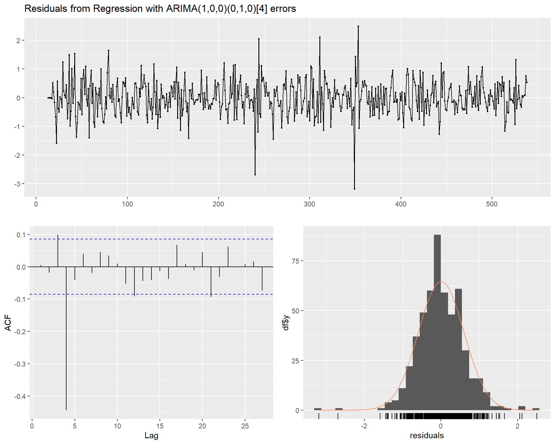
The result of the Ljung-Box test (1978) and the acf and pacf plots indicate statistically significant nonzero autocorrelation in the residuals. At this stage, however, the form of the noise is relatively unimportant. The main objective is to evaluate whether additional time differencing is required. As the residual errors from the regression model appear to be stationary, no further time differencing is required.
Let’s take a closer look at the acf and pacf plots.
acf(residuals(mod1))
pacf(residuals(mod1))
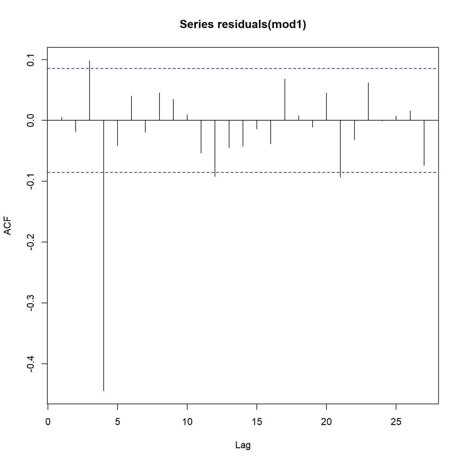
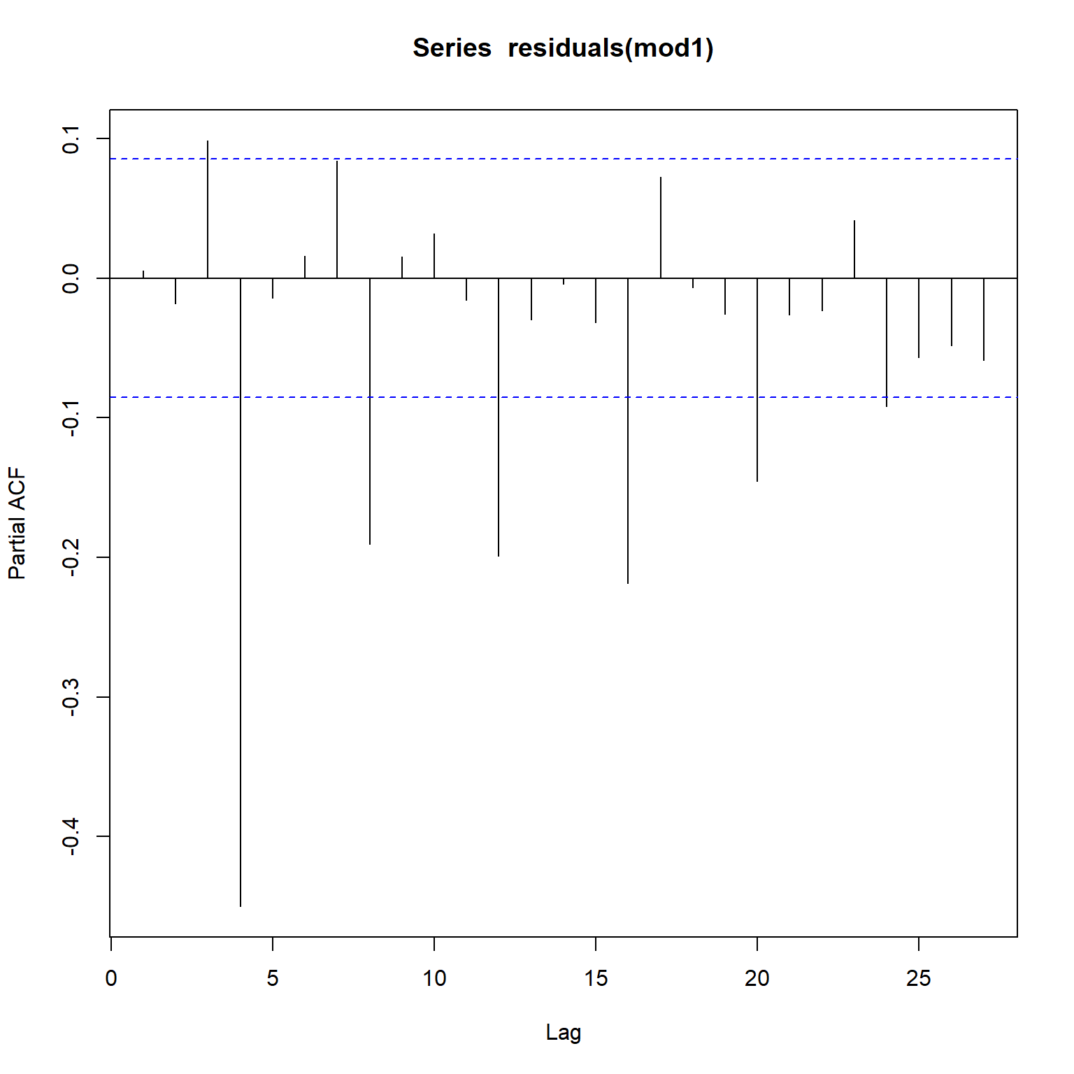
Both the acf and pacf plots indicate that the noise model is not appropriate. However, at this stage we have a large number of explanatory variables, so our first objective is to remove explanatory variables that are statistically non-significant.
Model 2
Let’s revise Model 1. Based on the coefficients of Model 1, it appears that lags higher than 2 are not important in capturing TCE response. Thus, we will revise Model 1 using a maximum lag of 2. The noise model still uses a low-order ARIMA model.
xr0.data <- cbind(
  radon0 = xy.ts[,2], radon1 = xy.ts[,3], radon2 = xy.ts[,4],
  DP0 = xy.ts[,13], DP1 = xy.ts[,14], DP2 = xy.ts[,15],
  DT0 = xy.ts[,24], DT1 = xy.ts[,25], DT2 = xy.ts[,26],
  TEMP0 = xy.ts[,35], TEMP1 = xy.ts[,36], TEMP2 = xy.ts[,37],
  WindSpeed0 = xy.ts[,39], WindSpeed1 = xy.ts[,40], WindSpeed2 = xy.ts[,41],
  BP0 = xy.ts[,43], BP1 = xy.ts[,44], BP2 = xy.ts[,45],
  Precip0 = xy.ts[,47], Precip1 = xy.ts[,48], Precip2 = xy.ts[,49],
  WH0 = xy.ts[,51], WH1 = xy.ts[,52], WH2 = xy.ts[,53],
  WD0 = xy.ts[,55], WD1 = xy.ts[,56], WD2 = xy.ts[,57]
)
mod2 <- arima(window(y.data, end = 538),
              xreg = window(xr0.data, end = 538),
              order = c(1, 0, 0),
              seasonal = list(order = c(0, 1, 0), period = 4))
mod2
##
## Call:
## arima(x = window(y.data, end = 538), order = c(1, 0, 0), seasonal = list(order = c(0,
##     1, 0), period = 4), xreg = window(xr0.data, end = 538))
##
## Coefficients:
##          ar1  radon0  radon1  radon2      DP0      DP1      DP2      DT0
##       0.2351  1.2019  0.1904  0.0347  -0.0641  -0.0516  -0.4675  -0.2253
## s.e.  0.0454  0.0574  0.0585  0.0585   0.0547   0.0551   0.3590   0.3507
##          DT1      DT2   TEMP0   TEMP1   TEMP2  WindSpeed0  WindSpeed1
##       0.1881  -0.1003  0.0075  0.0018  0.0092      0.0063     -0.0139
## s.e.  0.3646   0.3915  0.0100  0.0109  0.0080      0.0091      0.0089
##       WindSpeed2     BP0      BP1     BP2  Precip0  Precip1  Precip2     WH0
##          -0.0037  0.0130  -0.0135  0.0055   0.0095  -0.0074   0.0078  0.3244
## s.e.      0.0049  0.0049   0.0056  0.0059   0.0061   0.0068   0.0061  3.9184
##          WH1      WH2     WD0     WD1      WD2
##       2.3932  -6.0741  6.9228  0.0676  -0.1581
## s.e.  3.4090   3.4539  3.5133  0.1506   0.1530
##
## sigma^2 estimated as 0.3974:  log likelihood = -499.84,  aic = 1055.67
Let’s inspect the coefficients of Model 2. Based on these coefficients, it appears that the maximum lag can be further reduced to lag 1.
coeftest(mod2)
##
## z test of coefficients:
##
##              Estimate Std. Error z value  Pr(>|z|)
## ar1         0.2351422  0.0453821  5.1814 2.202e-07 ***
## radon0      1.2019203  0.0573688 20.9508 < 2.2e-16 ***
## radon1      0.1903537  0.0584992  3.2540  0.001138 **
## radon2      0.0347178  0.0584851  0.5936  0.552768
## DP0        -0.0641415  0.0546918 -1.1728  0.240883
## DP1        -0.0515695  0.0551462 -0.9351  0.349716
## DP2        -0.4674519  0.3589664 -1.3022  0.192842
## DT0        -0.2252649  0.3507246 -0.6423  0.520689
## DT1         0.1880825  0.3645916  0.5159  0.605944
## DT2        -0.1003448  0.3915205 -0.2563  0.797723
## TEMP0       0.0074866  0.0100366  0.7459  0.455709
## TEMP1       0.0018285  0.0109032  0.1677  0.866814
## TEMP2       0.0091967  0.0080195  1.1468  0.251466
## WindSpeed0  0.0063492  0.0091332  0.6952  0.486945
## WindSpeed1 -0.0139245  0.0089388 -1.5578  0.119290
## WindSpeed2 -0.0037240  0.0048567 -0.7668  0.443221
## BP0         0.0129883  0.0049037  2.6487  0.008081 **
## BP1        -0.0134908  0.0056183 -2.4012  0.016340 *
## BP2         0.0054699  0.0059209  0.9238  0.355575
## Precip0     0.0094928  0.0060520  1.5686  0.116752
## Precip1    -0.0074439  0.0068383 -1.0886  0.276348
## Precip2     0.0078376  0.0061482  1.2748  0.202383
## WH0         0.3243661  3.9183850  0.0828  0.934026
## WH1         2.3932447  3.4089706  0.7020  0.482652
## WH2        -6.0741198  3.4538647 -1.7586  0.078638 .
## WD0         6.9227578  3.5133166  1.9704  0.048789 *
## WD1         0.0676166  0.1506131  0.4489  0.653473
## WD2        -0.1581409  0.1530462 -1.0333  0.301469
## ---
## Signif. codes:  0 '***' 0.001 '**' 0.01 '*' 0.05 '.' 0.1 ' ' 1
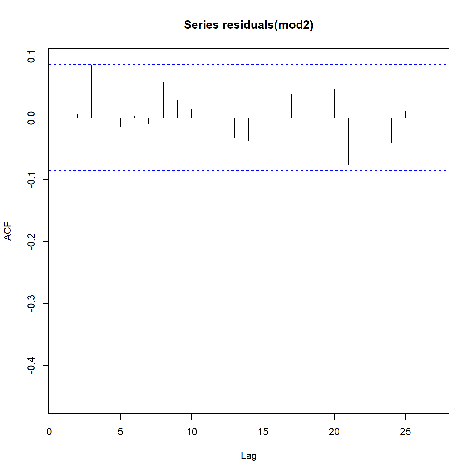
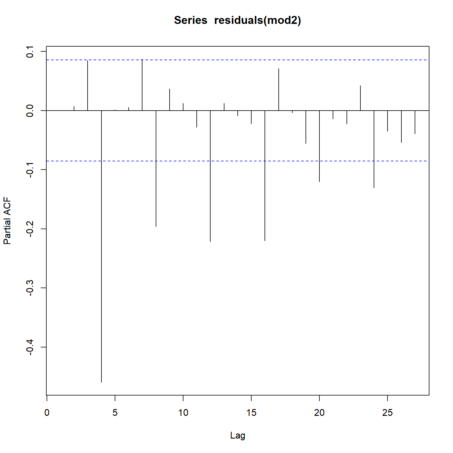
Let’s inspect the acf and pacf plots for Model 2. The residual errors remain very similar to those of the residual errors of Model 1. This indicates that it will be appropriate to add a seasonal MA component to model the noise appropriately.
acf(residuals(mod2))
pacf(residuals(mod2))
Model 3
To revise Model 2, two changes mentioned previously are made: (1) explanatory variables are reduced to lag 1 and (2) a seasonal MA component is added to the noise model.
xr1.data <- cbind(
  radon0 = xy.ts[,2], radon1 = xy.ts[,3],
  DP0 = xy.ts[,13], DP1 = xy.ts[,14],
  DT0 = xy.ts[,24], DT1 = xy.ts[,25],
  TEMP0 = xy.ts[,35], TEMP1 = xy.ts[,36],
  WindSpeed0 = xy.ts[,39], WindSpeed1 = xy.ts[,40],
  BP0 = xy.ts[,43], BP1 = xy.ts[,44],
  Precip0 = xy.ts[,47], Precip1 = xy.ts[,48],
  WH0 = xy.ts[,51], WH1 = xy.ts[,52],
  WD0 = xy.ts[,55], WD1 = xy.ts[,56]
)
mod3 <- arima(window(y.data,end=538), xreg = window(xr1.data,end=538), order = c(1, 0, 0),seasonal = list(order=c(0, 1, 1),period=4))
mod3
##
## Call:
## arima(x = window(y.data, end = 538), order = c(1, 0, 0), seasonal = list(order = c(0,
##     1, 1), period = 4), xreg = window(xr1.data, end = 538))
##
## Coefficients:
##          ar1     sma1  radon0  radon1      DP0      DP1      DT0     DT1
##       0.3423  -0.9114  1.1947  0.1421  -0.0457  -0.0478  -0.7744  0.1196
## s.e.  0.0432   0.0255  0.0564  0.0555   0.0555   0.0567   0.3477  0.3712
##        TEMP0   TEMP1  WindSpeed0  WindSpeed1     BP0      BP1  Precip0  Precip1
##       0.0042  0.0104      0.0103     -0.0067  0.0096  -0.0071   0.0129   0.0056
## s.e.  0.0077  0.0078      0.0079      0.0075  0.0042   0.0044   0.0061   0.0063
##           WH0     WH1     WD0     WD1
##       -1.9022  4.8319  4.5858  0.0954
## s.e.   3.1980  3.1241  3.0311  0.1577
##
## sigma^2 estimated as 0.2483:  log likelihood = -380.64,  aic = 801.28
Let’s inspect the coefficients of Model 3. Based on these coefficients, it appears that radon concentration (radon), barometric pressure (BP), precipitation (precip), and wind direction (WD) are important variables to explain variability in TCE concentration. Further, for radon and BP, both lag 0 and lag 1 are important, whereas, only lag 0 is important for precip and WD.
coeftest(mod3)
##
## z test of coefficients:
##
##              Estimate Std. Error  z value  Pr(>|z|)
## ar1         0.3423027  0.0432277   7.9186 2.402e-15 ***
## sma1       -0.9114250  0.0255172 -35.7180 < 2.2e-16 ***
## radon0      1.1946733  0.0564419  21.1664 < 2.2e-16 ***
## radon1      0.1420990  0.0555034   2.5602   0.01046 *
## DP0        -0.0456883  0.0555072  -0.8231   0.41045
## DP1        -0.0477619  0.0566655  -0.8429   0.39930
## DT0        -0.7744021  0.3476502  -2.2275   0.02591 *
## DT1         0.1195608  0.3711967   0.3221   0.74738
## TEMP0       0.0042203  0.0076803   0.5495   0.58267
## TEMP1       0.0104117  0.0077641   1.3410   0.17992
## WindSpeed0  0.0102935  0.0078589   1.3098   0.19026
## WindSpeed1 -0.0067124  0.0074708  -0.8985   0.36892
## BP0         0.0095976  0.0042100   2.2797   0.02262 *
## BP1        -0.0071449  0.0043638  -1.6373   0.10157
## Precip0     0.0128556  0.0061315   2.0966   0.03602 *
## Precip1     0.0056038  0.0062619   0.8949   0.37083
## WH0        -1.9021942  3.1979726  -0.5948   0.55197
## WH1         4.8319405  3.1241409   1.5466   0.12195
## WD0         4.5858462  3.0311416   1.5129   0.13030
## WD1         0.0953868  0.1576995   0.6049   0.54527
## ---
## Signif. codes:  0 '***' 0.001 '**' 0.01 '*' 0.05 '.' 0.1 ' ' 1
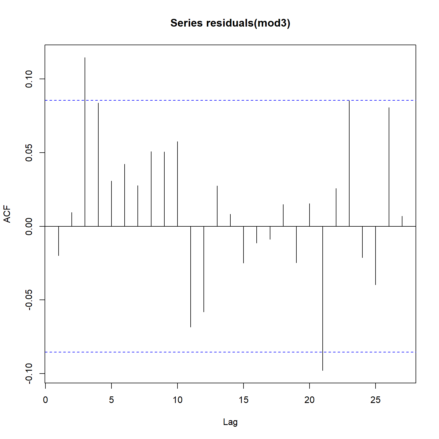
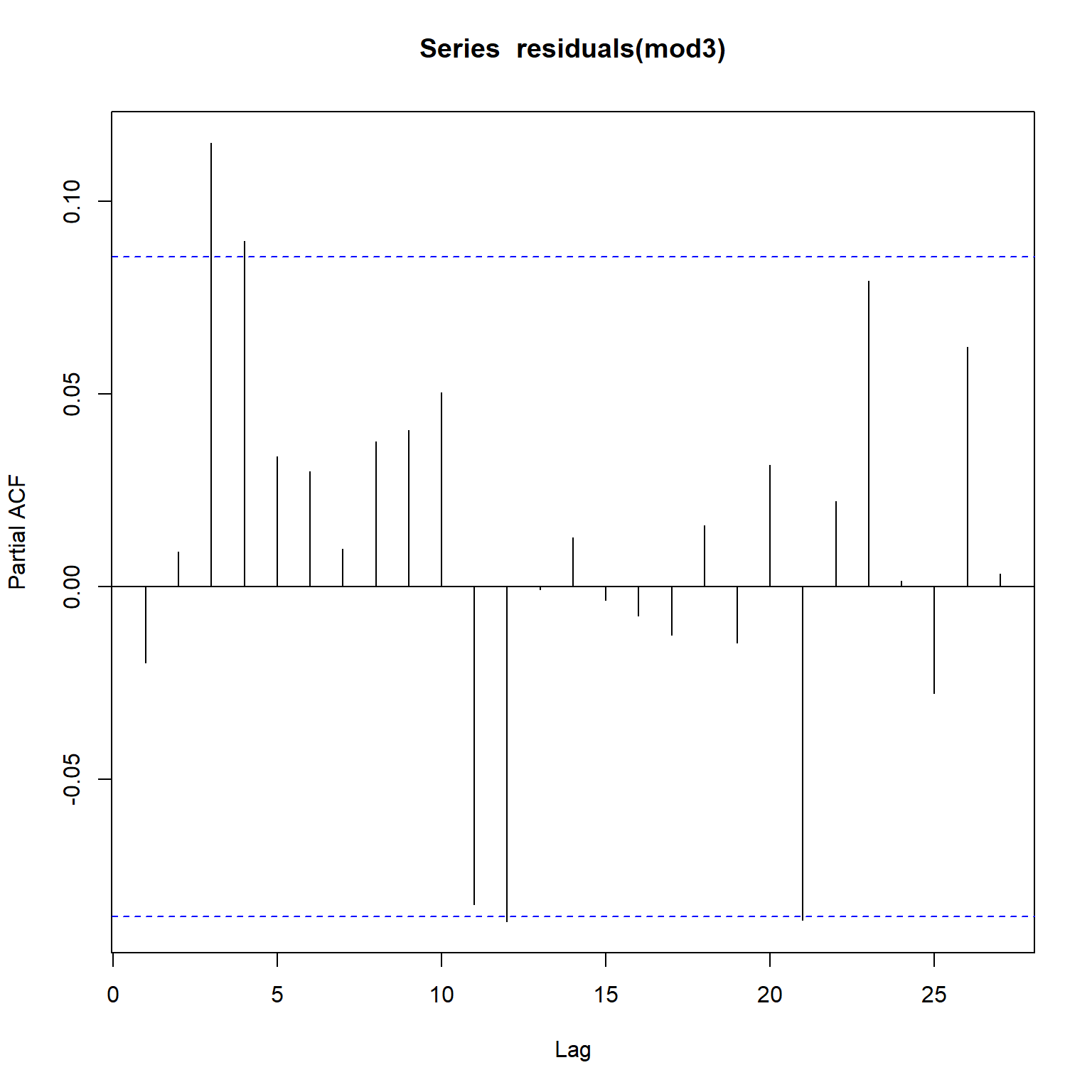
Inspecting the acf and pacf plots for Model 3, the seasonal autocorrelation has been adressed but a non-seasonal autocorrelation still persists in the residuals. It appears that addition of a higher-order AR component and an MA component is appropriate.
acf(residuals(mod3))
pacf(residuals(mod3))
Model 4
Let’s revise Model 3 using the following modifications: (1) retain Radon0, Radon1, BP0, BP1, Precip0, and WD0 as excogenous explanatory variables, and (2) use ARIMA(2,0,1)(0,1,1)[4] to model the residual errors.
xr2.data <- cbind(
  TCE0 = xy.ts[,1],
  radon0 = xy.ts[,2], radon1 = xy.ts[,3],
  BP0 = xy.ts[,43], BP1 = xy.ts[,44],
  Precip0 = xy.ts[,47],WD0 = xy.ts[,55]
)
mod4 <- Arima(window(xr2.data[,1], end = 538),
              xreg = window(xr2.data[,-1], end = 538),
              order = c(2, 0, 1),
              seasonal = list(order = c(0, 1, 1), period = 4))
mod4
## Series: window(xr2.data[, 1], end = 538)
## Regression with ARIMA(2,0,1)(0,1,1)[4] errors
##
## Coefficients:
##          ar1      ar2      ma1     sma1  radon0  radon1     BP0      BP1
##       1.0408  -0.1418  -0.7362  -0.9403  1.2095  0.1502  0.0122  -0.0078
## s.e.  0.1019   0.0649   0.0889   0.0210  0.0550  0.0545  0.0041   0.0042
##       Precip0     WD0
##        0.0104  4.7579
## s.e.   0.0054  2.9433
##
## sigma^2 = 0.2545:  log likelihood = -382.37
## AIC=786.75   AICc=787.27   BIC=833.58
Let’s inspect the coefficients of Model 4.
coeftest(mod4)
##
## z test of coefficients:
##
##           Estimate Std. Error  z value  Pr(>|z|)
## ar1      1.0408432  0.1019449  10.2099 < 2.2e-16 ***
## ar2     -0.1418298  0.0649197  -2.1847  0.028911 *
## ma1     -0.7361991  0.0888995  -8.2812 < 2.2e-16 ***
## sma1    -0.9403194  0.0210428 -44.6861 < 2.2e-16 ***
## radon0   1.2094885  0.0550375  21.9757 < 2.2e-16 ***
## radon1   0.1502233  0.0545163   2.7556  0.005859 **
## BP0      0.0122169  0.0041193   2.9658  0.003019 **
## BP1     -0.0077694  0.0042141  -1.8437  0.065232 .
## Precip0  0.0103551  0.0054202   1.9105  0.056074 .
## WD0      4.7579141  2.9432580   1.6165  0.105976
## ---
## Signif. codes:  0 '***' 0.001 '**' 0.01 '*' 0.05 '.' 0.1 ' ' 1
Let’s inspect the fitted model residuals and acf for Model 4. The scatter plot and histogram of the residual errors appear to be approximately white noise.
checkresiduals(mod4)
##
## 	Ljung-Box test
##
## data:  Residuals from Regression with ARIMA(2,0,1)(0,1,1)[4] errors
## Q* = 16.26, df = 3, p-value = 0.001003
##
## Model df: 10.   Total lags used: 13
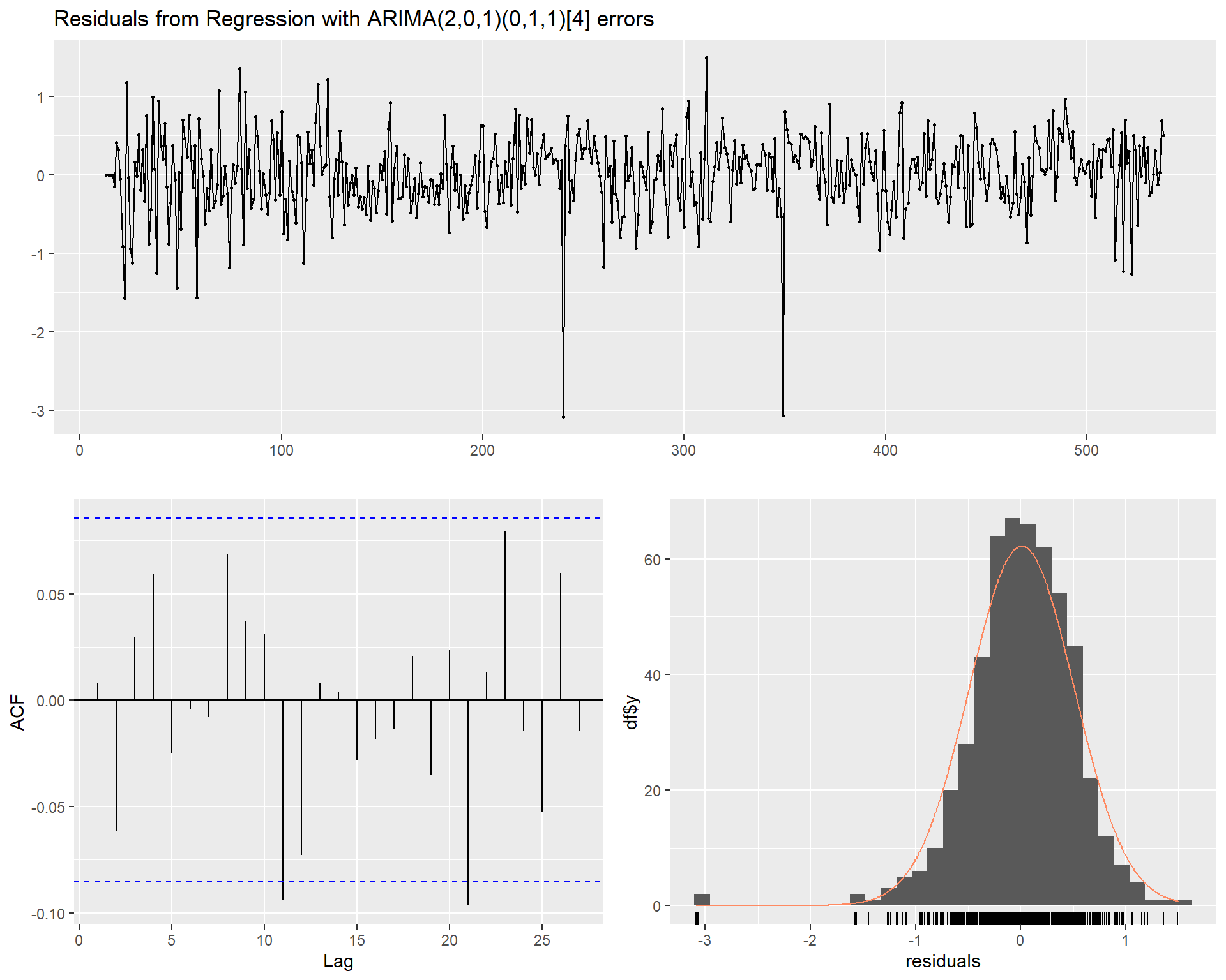
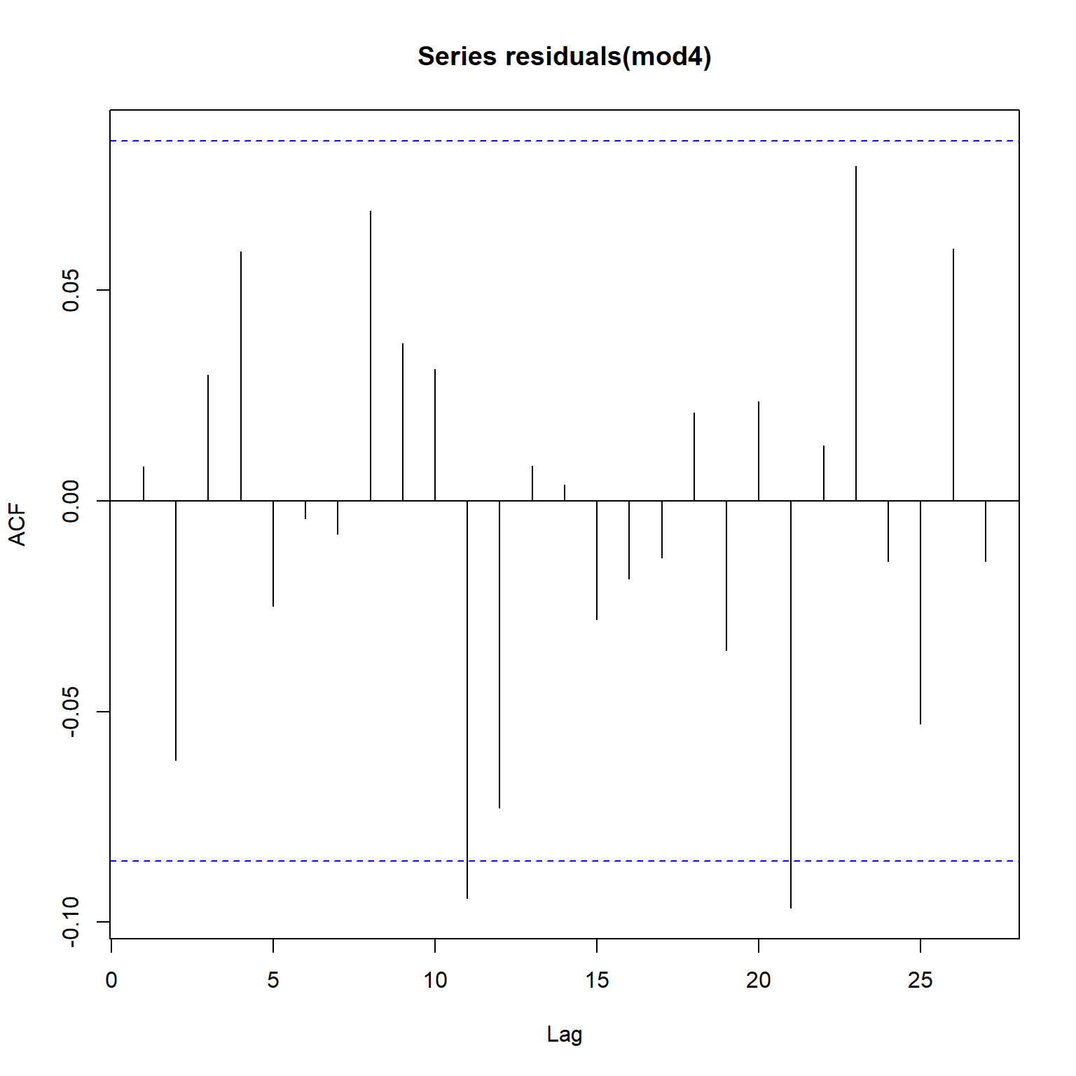
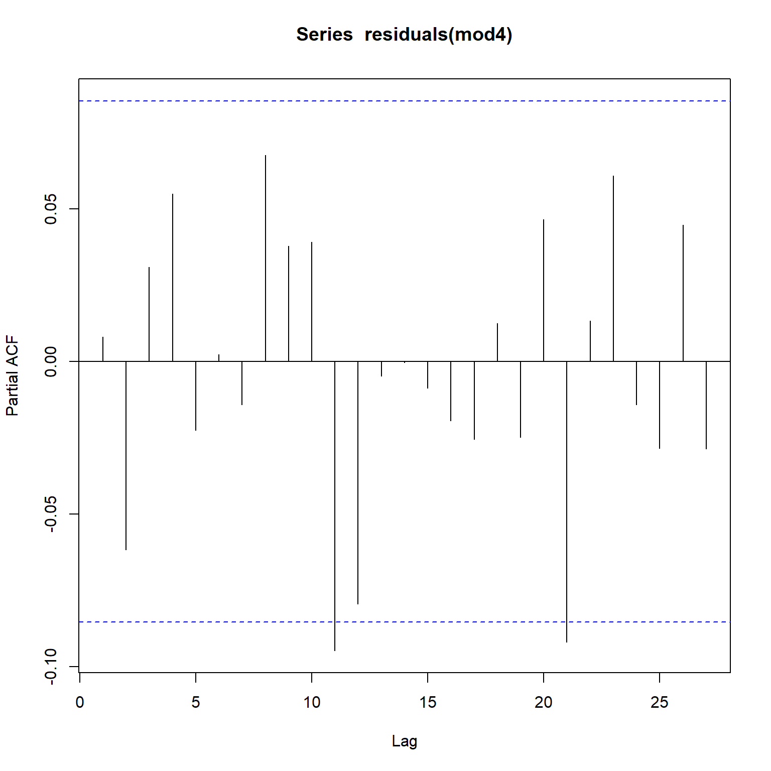
Based on the acf and pacf plots for Model 4 shown below, there is no evidence of any systematic autocorrelations in the residual series. The significant autocorrelations shown at lags 11 and 21 in the residual error do not appear to be systematic autocorrelations and hence can be ignored. Thus, Model 4 appears to be adequate.
acf(residuals(mod4))
pacf(residuals(mod4))
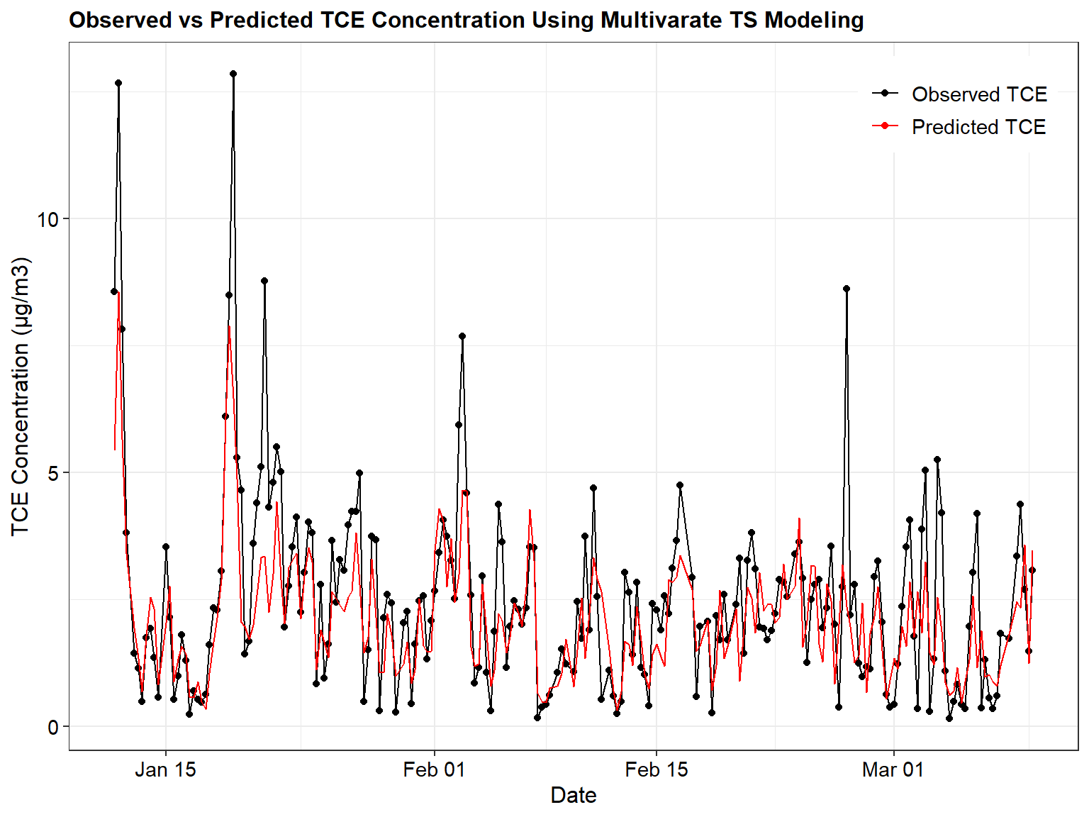
Let’s see how the predicted values for Model 4 compare to the actual observations.
# Comparison of observed results to predicted results
newfit2 <- Arima(xr2.data[,1], xreg = xr2.data[,-1], model = mod4)
result_df <- subset(dat, ObsNumber >= 15)
result_df$TSreg_Predicted <- fitted(newfit2)

ggplot(data = subset(result_df, ObsNumber >= 539),
       aes(x = Date)) +
  geom_point(aes(y = TCE,color = "Observed TCE")) +
  geom_line(aes(y = TCE,color = "Observed TCE")) +
  geom_line(aes(y = exp(TSreg_Predicted), color = "Predicted TCE")) +
  labs(title = "Observed vs Predicted TCE Concentration Using Multivarate TS Modeling",
       x = "Date",
       y = "TCE Concentration (µg/m3)") +
  scale_color_manual(breaks = c("Observed TCE",
                                "Predicted TCE"),
                     values = c("Observed TCE" = "black",
                                "Predicted TCE" = "red")) +
  theme_bw() +
  theme(plot.title = element_text(size = 12, hjust = 0, color = 'black', face = quote(bold)),
        axis.title.y = element_text(size = 12, color = 'black'),
        axis.title.x = element_text(size = 12, color = 'black'),
        axis.text.x = element_text(size = 11, color = 'black'),
        axis.text.y = element_text(size = 11, color = 'black'),
        legend.position = c(0.98, 0.98),
        legend.justification = c(1, 1),
        legend.title = element_blank(),
        legend.text = element_text(size = 11))
Conclusion
Several approaches have been proposed in the literature to select the best model specification. One of the most studied is the Akaike’s (1973) Information Criterion (AIC). The AIC is a single number score that can be used to determine which of multiple models is most likely to be the best model for a given dataset. The AIC score rewards models that achieve a high goodness-of-fit score and penalizes them if they become overly complex. It is an appropriate model selection criterion for models that are fitted using the maximum likelihood estimation framework. According to this criterion, the model that is selected minimizes: AIC = -2log(maximum likelihood) + 2k, where k = p + q + 1 if the model contains a constant (intercept) term, otherwise k = p + q. The model fit characteristics for the above four models are summarized below. It is clear from this table that Model 4 gives the minimum AIC score and hence is the best model.
| Model No. | Estimated Sigma^2 | Log Likelihood | AIC |
|---|---|---|---|
| 1 | 0.401 | -472 | 1,061 |
| 2 | 0.397 | -500 | 1,056 |
| 3 | 0.248 | -381 | 801 |
| 4 | 0.255 | -382 | 787 |
References
Akaike, H. 1973. Information theory and an extension of the maximum likelihood principle. In B. N. Petrov and F. Csaki, (eds.), 2nd International Symposium on Information Theory, Akademiai Kiado, Budapest.
Fuller, W. A. 1996. Introduction to Statistical Time Series, Second Edition. New York, John Wiley and Sons.
Hipel, K.W. and McLeod A. I. 1994. Time Series Modelling of Water Resources and Environmental Systems, Volume 45, 1st Edition, Elsevier Science, Amsterdam, The Netherlands.
Hyndman, R.J. and G. Athanasopoulos. 2013. Forecasting: Principles and Practice. Print edition. Heathmont, OTexts.
Ljung, G. and G. Box. 1978. On a measure of lack of fit in time series models. Biometrika, 65, 297-303.
- Posted on:
- May 13, 2020
- Length:
- 26 minute read, 5380 words
- See Also: