Introduction

The focus of trend analysis is on the long-term trend component over some multiyear period of interest. Methods for trend analysis are build on the basic concepts of regression analysis, including ordinary least squares (OLS) and nonparametric alternatives to OLS, in which the explanatory variable of interest is time. In most applications of trend analysis, the null hypothesis, \(H_0\), is that there is no trend (the data are independent and randomly ordered) in the variable being tested. The null hypothesis typically includes a set of assumptions related to the distribution of the data (normal versus non-normal), the type of trend (linear, monotonic, or step), and the degree of serial correlation. Failing to reject \(H_0\) does not prove there is no trend. Rather, it is a statement that given the available data and the assumptions of the particular test, there is not sufficient evidence to conclude that there is a trend.

Routine statistical methods for trend analysis cannot be directly applied for censored (containing non-detects) data. Substituting non-detects with arbitrary values, such as some fraction of the detection or reporting limit, prior to data analysis is generally a bias-prone approach. Substitution can introduce an invasive pattern to the data. For instance, if there is no change in detection limits over time, substitution can introduce a zero-slope pattern to the data. If detection limits are decreasing over time, substitution can introduce a false decreasing trend pattern to the data.

Statistical methods for dealing with censored data have a long history in the field of survival analysis and life testing (Helsel 2012). Six types of trend testing methods that can be used for censored data are presented in the table shown below. They are classified based on two factors. The first, shown in the rows of the table, is whether the test is parametric or nonparametric. The second factor, shown in the columns, is whether there is a need to remove variation caused by other associated variables. Variables other than time often have considerable influence on the response variable. These covariates are usually natural, random phenomena such as rainfall, temperature, groundwater elevation, or stream flow.

The objective of this post is to demonstrate the various methods that can be used to analyze censored environmental data for temporal trend. Trend testing will be conducted using the NADA2 library for R. The NADA2 library includes methods for plotting, computing summary statistics, hypothesis testing, and developing regression models for data with one or more detection limits. This library consists of new procedures and improvements on current procedures contained in the NADA library.

Libraries

We’ll start by loading the R libraries required for data manipulation, exploration, visualization, and modelling.

# Load libraries
library(NADA2)
library(survival)
library(car)

Data

The data consist of total recoverable chromium (TCr) concentrations in stream flows of Gales Creek in Oregon, USA. Concentration and daily stream flow (discharge) were measured by season (wet versus dry) between January 2009 and October 2018. Concentrations are given in micrograms per liter (µ/L) and include censored values with two detection limits.

# Load data
data(Gales_Creek)

# Inspect structure of data
str(Gales_Creek)
## tibble [63 × 11] (S3: tbl_df/tbl/data.frame)
##  $ Date     : POSIXct[1:63], format: "2009-01-06" "2009-02-03" ...
##  $ Yr       : num [1:63] 2009 2009 2009 2009 2009 ...
##  $ Month    : chr [1:63] "January" "February" "March" "April" ...
##  $ Season   : chr [1:63] "Wet" "Wet" "Wet" "Wet" ...
##  $ Descript : chr [1:63] "GALES CREEK AT NEW HWY 47" "GALES CREEK AT NEW HWY 47" "GALES CREEK AT NEW HWY 47" "GALES CREEK AT NEW HWY 47" ...
##  $ Units    : chr [1:63] "µg/L" "µg/L" "µg/L" "µg/L" ...
##  $ Flag     : chr [1:63] NA NA NA "<" ...
##  $ TCr      : num [1:63] 2.76 0.836 1.88 0.6 3.99 0.544 1.35 0.6 0.6 0.6 ...
##  $ discharge: num [1:63] 742 140 301 196 341 74 26 9.5 18 19 ...
##  $ CrND     : num [1:63] 0 0 0 1 0 0 0 1 1 1 ...
##  $ dectime  : num [1:63] 2009 2009 2009 2009 2009 ...

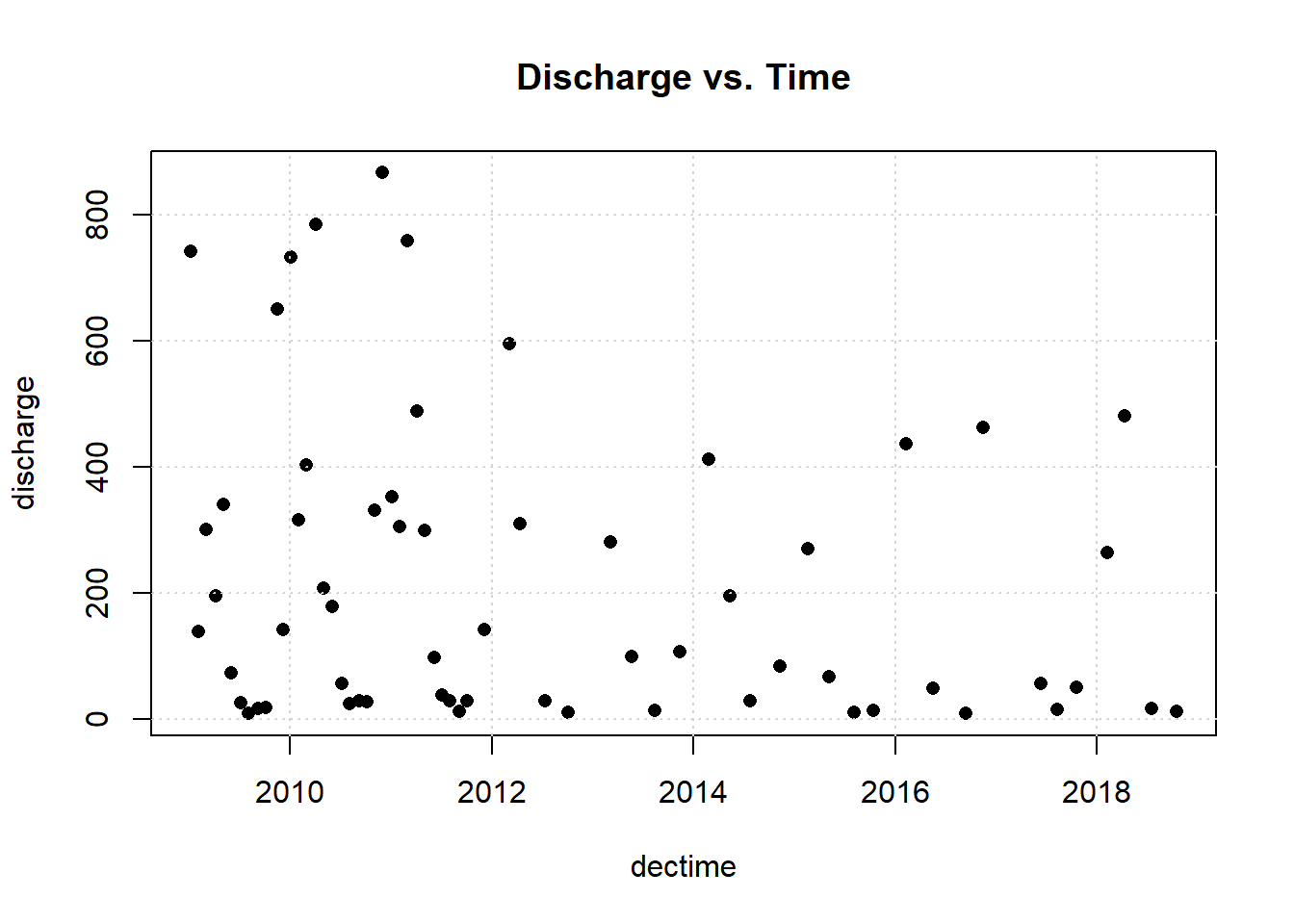
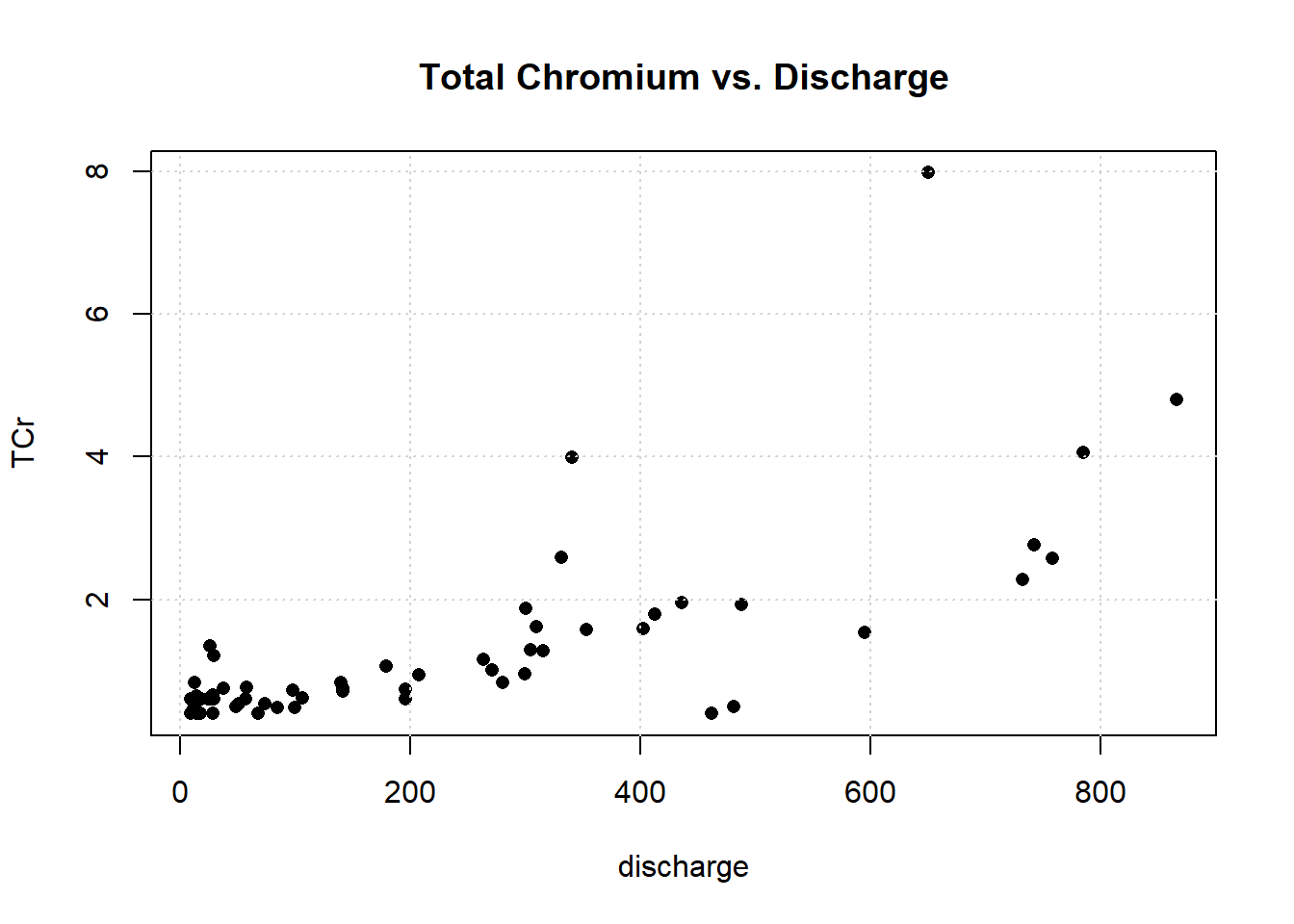
Let’s plot the data.

# Plot data
with(Gales_Creek,
  plot(
    dectime, TCr,
    pch = 16, cex = 1,
    main = 'Total Chromium vs. Time'
  )
)
grid()
with(Gales_Creek,
  plot(
    dectime, discharge,
    pch = 16, cex = 1,
    main = 'Discharge vs. Time'
  )
)
grid()
with(Gales_Creek,
  plot(
    discharge, TCr,
    pch = 16, cex = 1,
    main = 'Total Chromium vs. Discharge'
  )
)
grid()

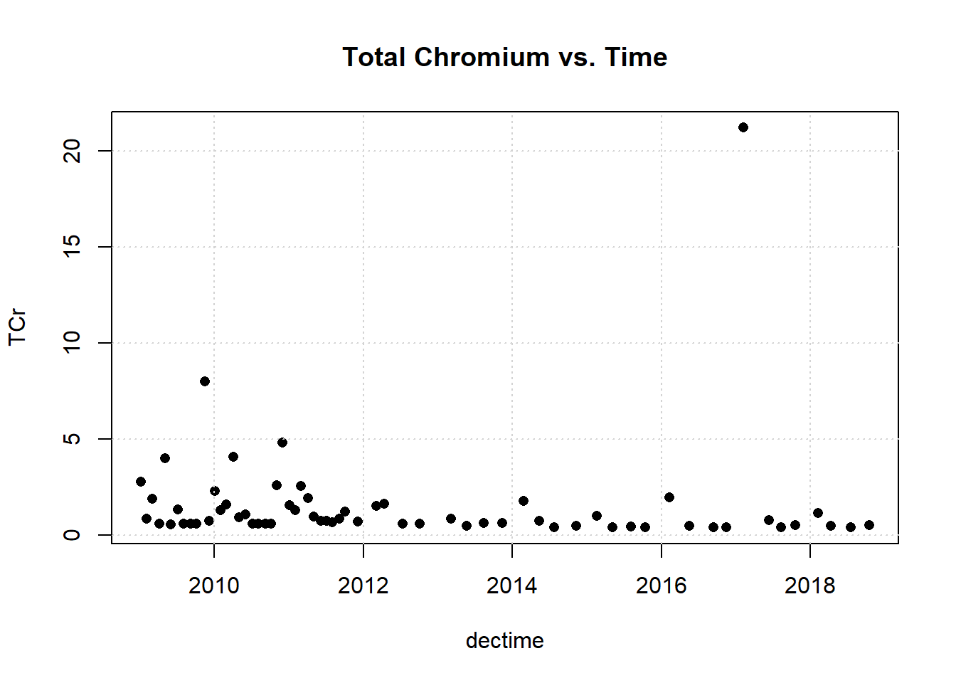
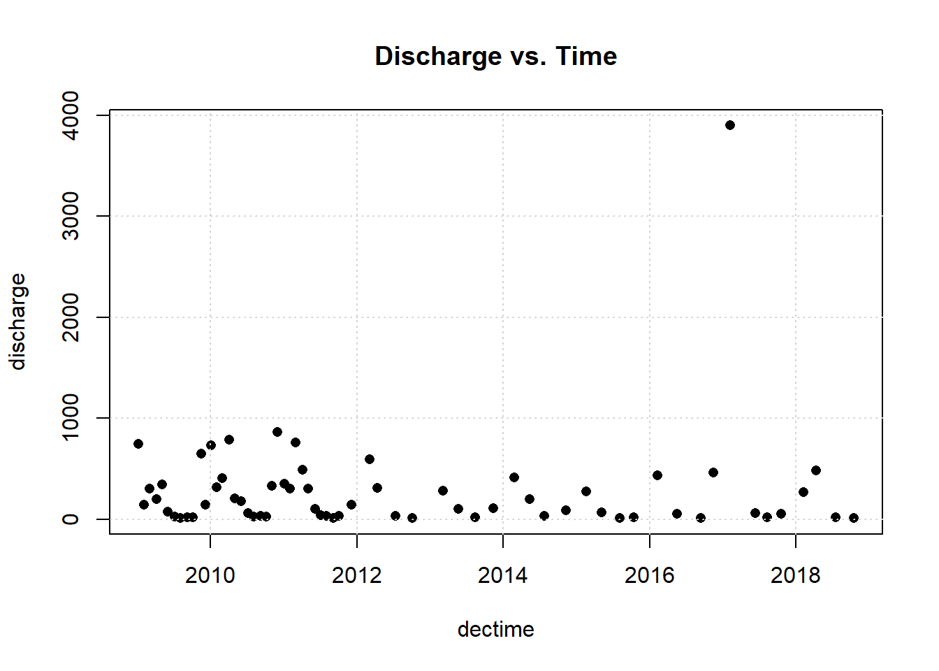
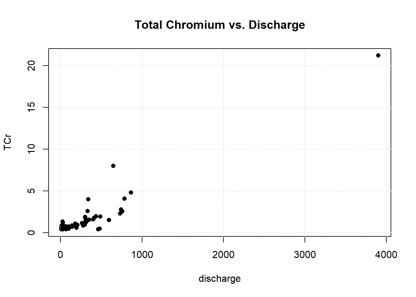
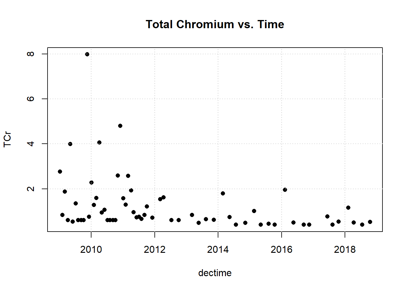
One observation appears to be far removed from the remaining portion of the data. Let’s remove the outlying observation and re-plot the data.

# Remove suspected outlier
idx <- which.max(Gales_Creek$TCr)
dat <- Gales_Creek[-idx,]

# Plot data with outlier removed
with(dat,
  plot(
    dectime, TCr,
    pch = 16, cex = 1,
    main = 'Total Chromium vs. Time'
  )
)
grid()
with(dat,
  plot(
    dectime, discharge,
    pch = 16, cex = 1,
    main = 'Discharge vs. Time'
  )
)
grid()
with(dat,
  plot(
    discharge, TCr,
    pch = 16, cex = 1,
    main = 'Total Chromium vs. Discharge'
  )
)
grid()

Parametric Methods

There are several methods for incorporating censored observations into linear models. Maximum likelihood estimates of slope and intercept produce a parametric regression model without the use of substitution.

MLE Simple Regression (Time Only)

Maximum likelihood estimation (MLE) assumes the data have a particular shape (or distribution). The method fits a distribution to the data that matches both the values for detected observations, and the proportion of observations falling below each detection limit. The information contained in non-detects is captured by the proportion of data falling below each detection limit. Because the model uses the parameters of a probability distribution, MLE is a fully parametric approach and all inference is based on the assumed distribution. A limitation of MLE is that the residuals from the regression (bivariate residuals for correlation) must follow a chosen distribution, and the data sample size should be large enough to enable verification that the assumed data distribution is reasonable.

Let’s perform MLE for simple linear regression using time as an explanatory variable.

# Simple regression using time as explanatory variable.
reg1 <- with(dat, cencorreg(TCr, CrND, dectime, LOG = TRUE))
##  Likelihood R = -0.4074                     AIC = 143.2094 
## Rescaled Likelihood R = -0.4278            BIC = 148.6388 
##  McFaddens R = -0.2763 
## 
summary(reg1)
## 
## Call:
## survreg(formula = "log(TCr)", data = "dectime", dist = "gaussian")
##                Value Std. Error     z      p
## (Intercept) 259.6388    73.3848  3.54 0.0004
## dectime      -0.1291     0.0365 -3.54 0.0004
## Log(scale)   -0.2429     0.1116 -2.18 0.0295
## 
## Scale= 0.784 
## 
## Gaussian distribution
## Loglik(model)= -68.1   Loglik(intercept only)= -73.7
## 	Chisq= 11.26 on 1 degrees of freedom, p= 0.00079 
## Number of Newton-Raphson Iterations: 4 
## n= 62

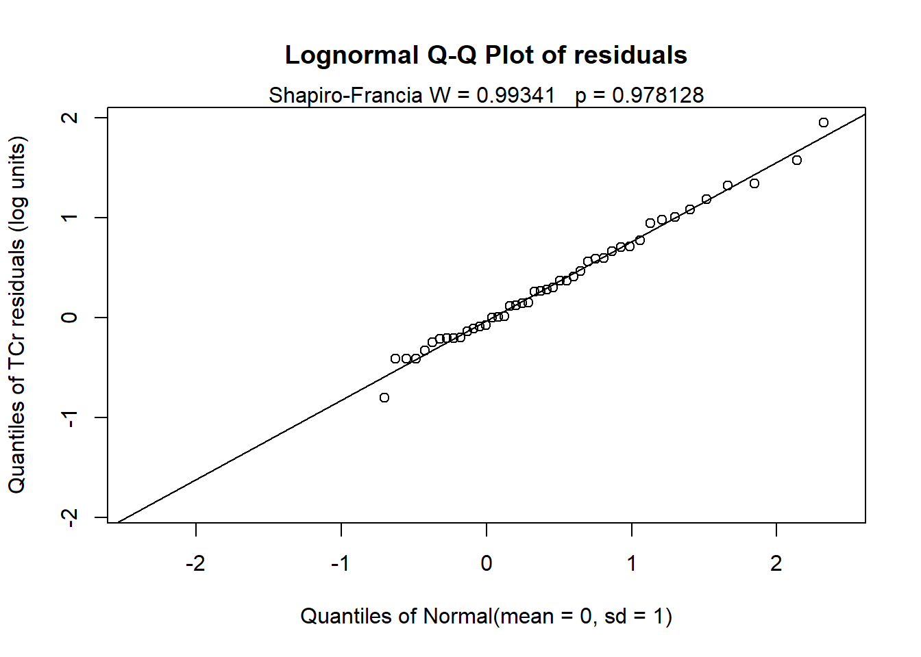
The Q-Q plot of the residuals using log(TCr) and the results of the Shapiro-Francia test indicate that normality of the residuals is a valid assumption. The model is statistically significant (p = 0.0008) showing a downward trend in TCr concentrations of 0.129 log units per year.

MLE Multiple Regression (Time + Covariate)

Now, let’s perform MLE for multiple regression using both discharge and time as explanatory variables. To do multiple regression using the cencorreg() function, we need to input the x variables as a single data frame.

xvar <- data.frame(dectime = dat$dectime, discharge = dat$discharge)
reg2 <- with(dat, cencorreg(TCr, CrND, xvar))
##  Likelihood R2 = 0.6533                     AIC = 90.79285 
##  Rescaled Likelihood R2 = 0.72            BIC = 98.36539 
##  McFaddens R2 = 0.4453 
## 
summary(reg2)
## 
## Call:
## survreg(formula = "log(TCr)", data = "dectime+discharge", dist = "gaussian")
##                 Value Std. Error     z       p
## (Intercept)  1.50e+02   4.39e+01  3.41 0.00065
## dectime     -7.48e-02   2.18e-02 -3.43 0.00061
## discharge    2.48e-03   2.66e-04  9.33 < 2e-16
## Log(scale)  -7.95e-01   1.10e-01 -7.25   4e-13
## 
## Scale= 0.452 
## 
## Gaussian distribution
## Loglik(model)= -40.9   Loglik(intercept only)= -73.7
## 	Chisq= 65.67 on 2 degrees of freedom, p= 5.5e-15 
## Number of Newton-Raphson Iterations: 6 
## n= 62

Similiar to MLE for simple regression, the Q-Q plot of the residuals using log(TCr) and the results of the Shapiro-Francia test indicate that normality of the residuals is a valid assumption. Both time and discharge are statistically significant, with a downward trend in TCr concentrations of 0.075 log units per year, adjusted for discharge, and increasing TCr concentrations with higher discharge.

Akaike’s Information Criterion (AIC) is a metric used to compare the fit of different regression models. Basically, it performs a cost-benefit analysis on the addition of variables to an equation. Adding a variable introduces a cost, which may or may not be offset by a reduction in the residual noise unexplained by the model. The best model is the one with the lowest AIC for a given dataset. The AIC for the two-variable (time + discharge) model is lower than for the single-variable (time only) model, indicating that the two-variable model is better.

Standard errors and hence the variances of the estimated coefficients are inflated when multicollinearity exists between explanatory variables in a model. The variance inflation factor (VIF) is a measure of collinearity among explanatory variables within a multiple regression. It is calculated by taking an independent variable and regressing it against every other explanatory variable in the model. The general rule of thumb is that VIFs exceeding 10 are signs of serious multicollinearity requiring correction. We can check the VIFs using the vif() function in the car library.

vif(lm(TCr ~ dectime + discharge, data = dat))
##   dectime discharge 
##  1.057955  1.057955

The VIFs for both time and discharge are well below 10.

MLE Multiple Regression With Seasonality (Time + Covariate + Seasonal)

One way to model seasonality and trend is to describe the seasonal patterns by a trigonometric regression using sine and cosine so one year is a full cycle of the trigonometric term. To accomplish this, we will add two new explanatory variables to the regression equation. These are the sine and cosine of \(2*pi*T\), where T is time in decimal years. Recall that for the cencorreg() function, we need to input the x variables as a single data frame.

# Add seasonal terms
cosT <- cos(2*pi*dat$dectime)
sinT <- sin(2*pi*dat$dectime)

# Input the x variables as a single data frame.
xvar2 <- data.frame(
  dectime = dat$dectime,
  discharge = dat$discharge,
  sinT, cosT
)
reg3 <- with(dat, cencorreg(TCr, CrND, xvar2))
##  Likelihood R2 = 0.6562                     AIC = 94.26963 
##  Rescaled Likelihood R2 = 0.7232            BIC = 106.1284 
##  McFaddens R2 = 0.4489 
## 

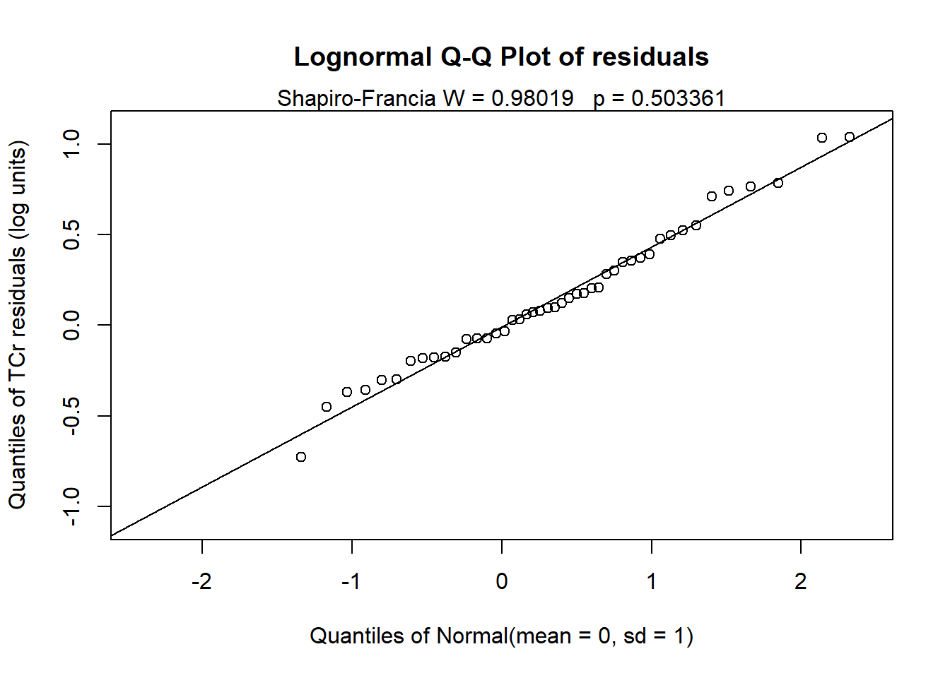
The Q-Q plot of the residuals using log(TCr) and the results of the Shapiro-Francia test indicate that normality of the residuals is a valid assumption. The AIC for this model is higher than the AC obtained for the two-variable model, indicating the two-variable model is better (i.e., no significant seasonal variation).

Let’s check for collinearity between the explanatory variables using the vif() function in the car library.

with(dat, car::vif(lm(TCr ~ dectime + discharge + sinT + cosT)))
##   dectime discharge      sinT      cosT 
##  1.062055  2.168696  1.393790  1.673697

The VIFs are satisfactory. Now, let’s fit a parametric survival regression model using time, discharge, and seasonality.

# Fit a parametric survival regression model
dat$TCr.Left <- ifelse(dat$CrND == 1, -Inf, dat$TCr)
survdat <- with(dat, Surv(TCr.Left, TCr, type = 'interval2'))
reg4 <- survreg(
  survdat ~ dectime + discharge + sinT + cosT,
  data = dat,
  dist = 'lognormal'
)
summary(reg4)
## 
## Call:
## survreg(formula = survdat ~ dectime + discharge + sinT + cosT, 
##     data = dat, dist = "lognormal")
##                 Value Std. Error     z       p
## (Intercept)  1.52e+02   4.43e+01  3.42 0.00063
## dectime     -7.56e-02   2.20e-02 -3.44 0.00059
## discharge    2.30e-03   3.68e-04  6.24 4.5e-10
## sinT         4.85e-02   9.85e-02  0.49 0.62242
## cosT         7.37e-02   1.13e-01  0.65 0.51268
## Log(scale)  -7.92e-01   1.10e-01 -7.21 5.7e-13
## 
## Scale= 0.453 
## 
## Log Normal distribution
## Loglik(model)= -47   Loglik(intercept only)= -80.1
## 	Chisq= 66.2 on 4 degrees of freedom, p= 1.4e-13 
## Number of Newton-Raphson Iterations: 6 
## n= 62

We see that both time and discharge are statistically significant. The model indicates a downward trend in TCr concentrations of 0.076 log units per year, adjusted for discharge, and increasing TCr concentrations with higher discharge. The seasonal terms are not statistically significant.

Nonparametric Methods

A variation of the Thiel-Sen line can be utilized for nonparametric trend analysis of censored data.

Simple Nonparametric Regression (Time Only)

A nonparametric method that is not affected by non-detects is to perform censored regression on the data, where the best-fit line for trend is computed using the Akritas-Theil-Sen (ATS) nonparametric line with the Turnbull estimate for intercept (Turnbull 1976). Akritas et al. (1995) extended the Theil-Sen method to censored data by calculating the slope that, when subtracted from the y data, would produce an approximately zero value for the Kendall’s tau correlation coefficient. The significance test for the ATS slope is the same test as that for the Kendall’s tau correlation coefficient (Helsel 2012). When the explanatory variable is a measure of time, the significance test for the slope is a test for (temporal) trend.

As a nonparametric test, ATS makes no assumption about the distribution of the residuals of the data; however, computing a slope implies that the data follow a linear pattern. If the data do not follow a linear pattern, either the Y or X variables should be transformed to produce a linear pattern before a slope is computed. Otherwise, the statement that a single slope describes the change in value for data in the original units is incorrect.

The ATS() function in the NADA2 library computes Kendall’s tau and the ATS line for censored data, along with the test that the slope (and Kendall’s tau) equal zero.

# Akritas-Theil-Sen line for censored data
with(dat, ATS(TCr, CrND, dectime, LOG = FALSE))
## Akritas-Theil-Sen line for censored data 
##  
## TCr = 208.7106 -0.1033 * dectime 
## Kendall's tau = -0.2671   p-value = 0.00205 
## 

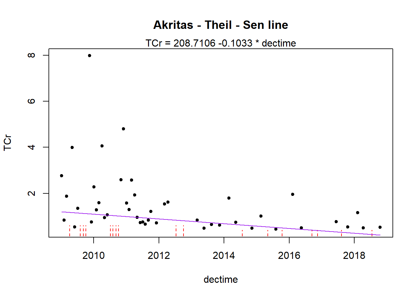
The model is linear over time with a statistically significant (p = 0.002) downward trend. There is a median decrease in TCr concentrations of 0.103 units per year.

The plot shows the TCr concentrations as a function of sample collection date where non-detects are shown as red, dashed vertical lines extending from zero to the detection limit and detects are shown as single points. Because censored values are known to be within an interval between zero and the censoring limit, representing these values by an interval provides a visual depiction of what is actually known about the data.

Multiple Nonparametric Regression (Time + Covariate)

For this approach to trend testing, we first remove the influence of the covariate on the response variable and then conduct a test for trend on the residuals. A generalized additive model (GAM) is used to find a smooth response function to model the relationship between the response variable and the covariate. The residuals of the model are then used to fit an ATS line and conduct Kendall’s tau test of change in residuals over time. The slope is given in the units of the response variable per time.

The centrend() function in the NADA2 library computes the ATS line and trend test for censored data after adjustment for a covariate. The default GAM smoother used in the centrend() function is a cubic regression spline with shrinkage.

# Use centrend() function
resid.trend <- with(dat,
  centrend(
    y.var = TCr,
    y.cens = CrND,
    x.var = discharge,
    time.var = dectime,
    Smooth = 'cs',
    stackplots = TRUE
  )
)
## Trend analysis of TCr adjusted for discharge 
## Akritas-Theil-Sen line for censored data 
##  
## TCr residuals = 89.1882 -0.0443 * dectime 
## Kendall's tau = -0.0709   p-value = 0.41763 
## 

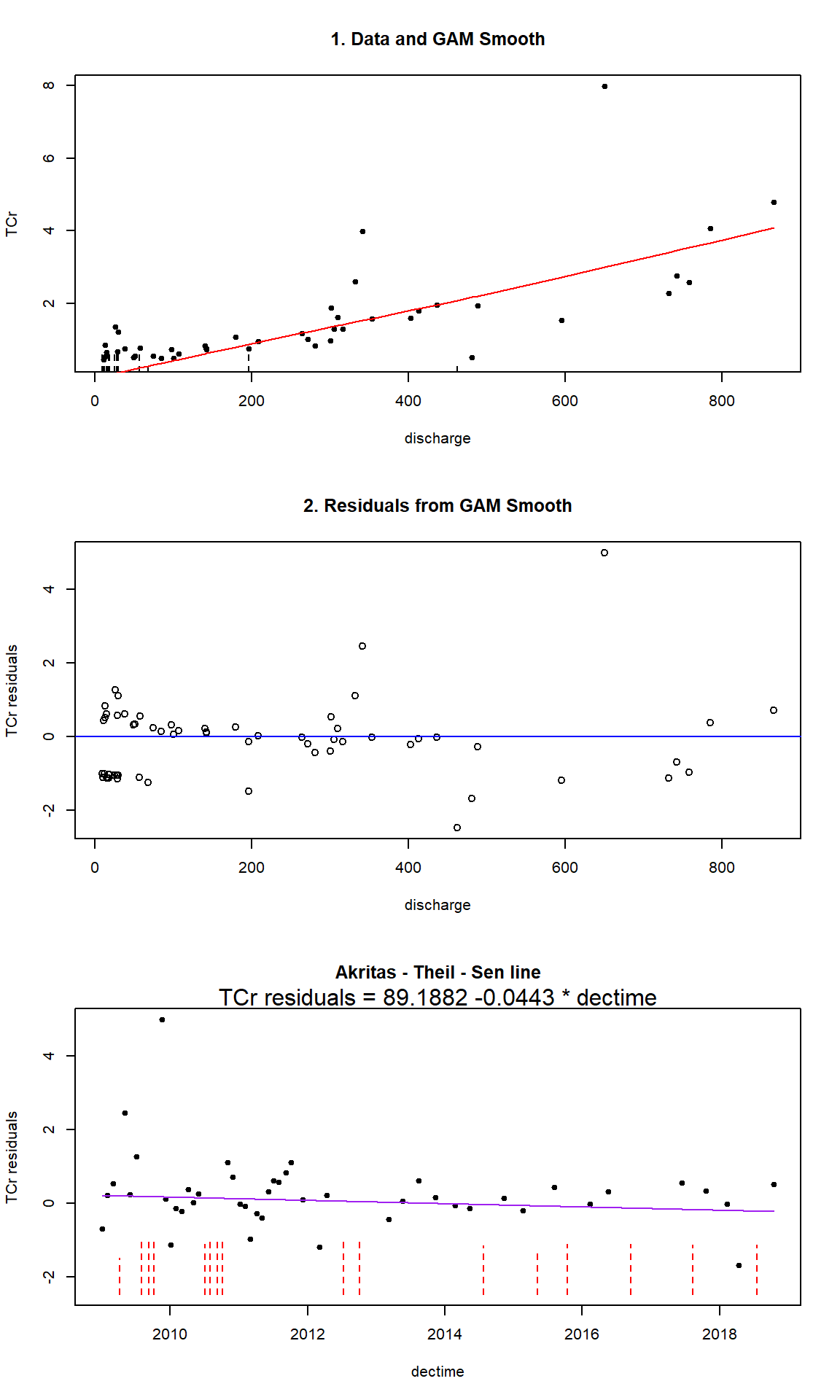
The model is not statistically significant (p = 0.418), indicating we cannot reject the null hypothesis of zero slope in TCr concentrations over time after adjustment for discharge.

Seasonal Kendall Test (Time + Seasonal)

The Seasonal Kendall (SK) test accounts for seasonality by computing an ATS line and test for each season separately and then combining the results. The test compares all data within the same season to one another but does not compare data across different seasons. The individual S test statistic for each season are combined to get an overall SK test result. If one season exhibits a significant increasing trend and a second season exhibits a significant decreasing trend, these may cancel each other out so that there is no overall significant SK trend. When there is an important covariate present, the SK test can be performed on residuals from a GAM of Y as a function of X, where X is not time.

The censeaken() function in the NADA2 library computes a SK permutation test on censored data with no covariate.

# Use censeaken() function
par(mfrow = c(2, 2))
with(dat,
  censeaken(
    time = dectime,
    y = TCr,
    y.cen = CrND,
    group = Season,
    seaplots = TRUE
  )
)
## 
##  DATA ANALYZED: TCr vs dectime by Season 
## ----------
##   Season  N    S    tau     pval Intercept    slope
## 1    Dry 34 -120 -0.214 0.069046    101.24 -0.05001
## ----------
##   Season  N    S    tau     pval Intercept   slope
## 1    Wet 28 -107 -0.283 0.036134    296.37 -0.1466
## ---------- 
## Seasonal Kendall test and Theil-Sen line
##   reps_R  N S_SK tau_SK   pval intercept   slope
## 1   4999 62 -227 -0.242 0.0042    208.71 -0.1033
## ----------

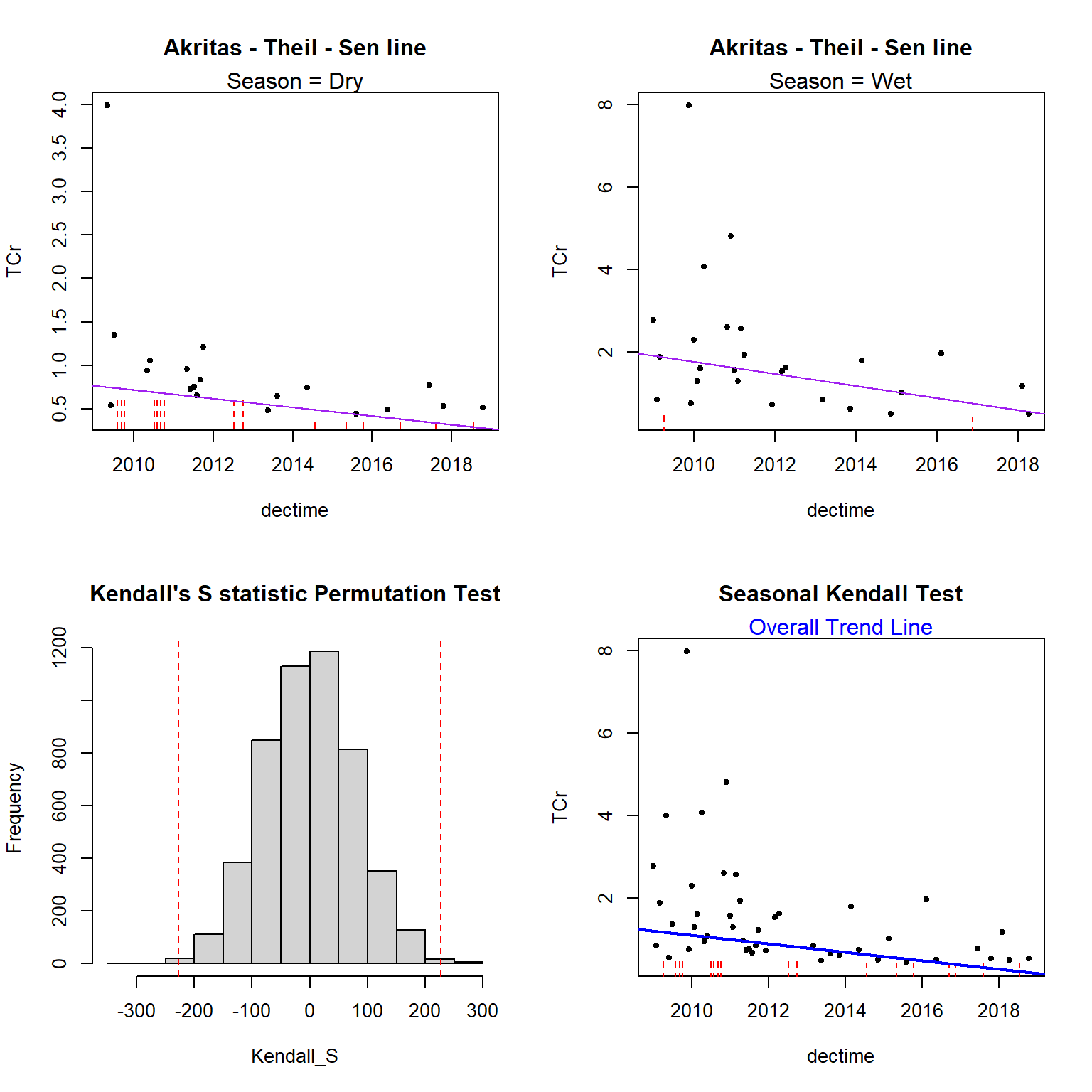
The results indicate a statistically significant downward trend (p = 0.036) in the Wet season and a weak, but suggestive, evidence of a downward trend (p = 0.069) in the Dry season. There is a statistically significant downward trend (p = 0.002) overall with a SK slope of -0.103 units per year.

Summary

This post examined several methods for conducting temporal trend analysis using censored data that do not substitute artificial values for non-detects. Parametric methods are based on censored regression using MLE. Nonparametric methods are based on Kendall’s tau and the Akritas-Theil-Sen line. The particular method used should be based on the characteristics of the data and whether there is a need to remove variation caused by other associated variables.

References

Akritas, M.G., Murphy, S.A., Lavalley, M.P., 1995. The Theil-Sen estimator with doubly censored data and applications to astronomy. J. Am. Stat. Assoc. 90, 170-177.

Helsel, D. R. 2012. Statistics for Censored Environmental Data using Minitab and R, 2nd edition. New York: John Wiley & Sons.

Sen, P.K. 1968. Estimates of the regression coefficient based on Kendall’s tau. J. Am. Stat. Assoc. 63, 1379-1389.

Theil, H. 1950. A rank-invariant method of linear and polynomial regression analysis. Nederl. Akad. Wetensch, Proceed. 53, 386-392.

Turnbull, B.W., 1976. The empirical distribution function with arbitrarily grouped, censored andtruncated data. J. Royal Stat. Soc. Ser. B Methodol. 38, 290-295.