Introduction

The most common activity in research is the comparison of two groups. If the data in each group are normally distributed, a two-sample t-test can be used to compare the means of the two groups. If these assumptions are severely violated, the nonparametric Wilcoxon Rank Sum (WRS) test, the randomization test, or the Kolmogorov-Smirnov test may be considered instead. One of the reasons for the popularity of the t-test, particularly the Aspin-Welch Unequal-Variance t-test, is its robustness in the face of assumption violation. However, if an assumption is not met even approximately, the significance levels and the power of the test may be significantly impacted. The t-test is robust to departures from normally, if the distributions are symmetric. That is, the test works as long as the distributions are symmetric, similar to that of a normal distribution, but performance may be affected if the distribution is asymmetric.

Simulating Performance

Using computer simulations, we will examine the robustness of the t-test under different conditions. We will compare the null hypothesis that two groups both have mean 100 to the alternative hypothesis that one group has mean 100 and the other has mean 110. We’ll assume both distributions have a standard deviation of 15 and for simplicity, we will maintain equal variance in both groups. Each group will be comprised of 36 independent, random samples.

The simulations will be conducted using a 5% significance level and 80% power. Under the null hypothesis, when the two groups come from the same distribution, we expect the test to wrongly conclude that the two distributions are different 5% of the time. Under the alternative hypothesis, when the two groups come from different distributions, we expect the test to conclude that the two means are indeed different 80% of the time.

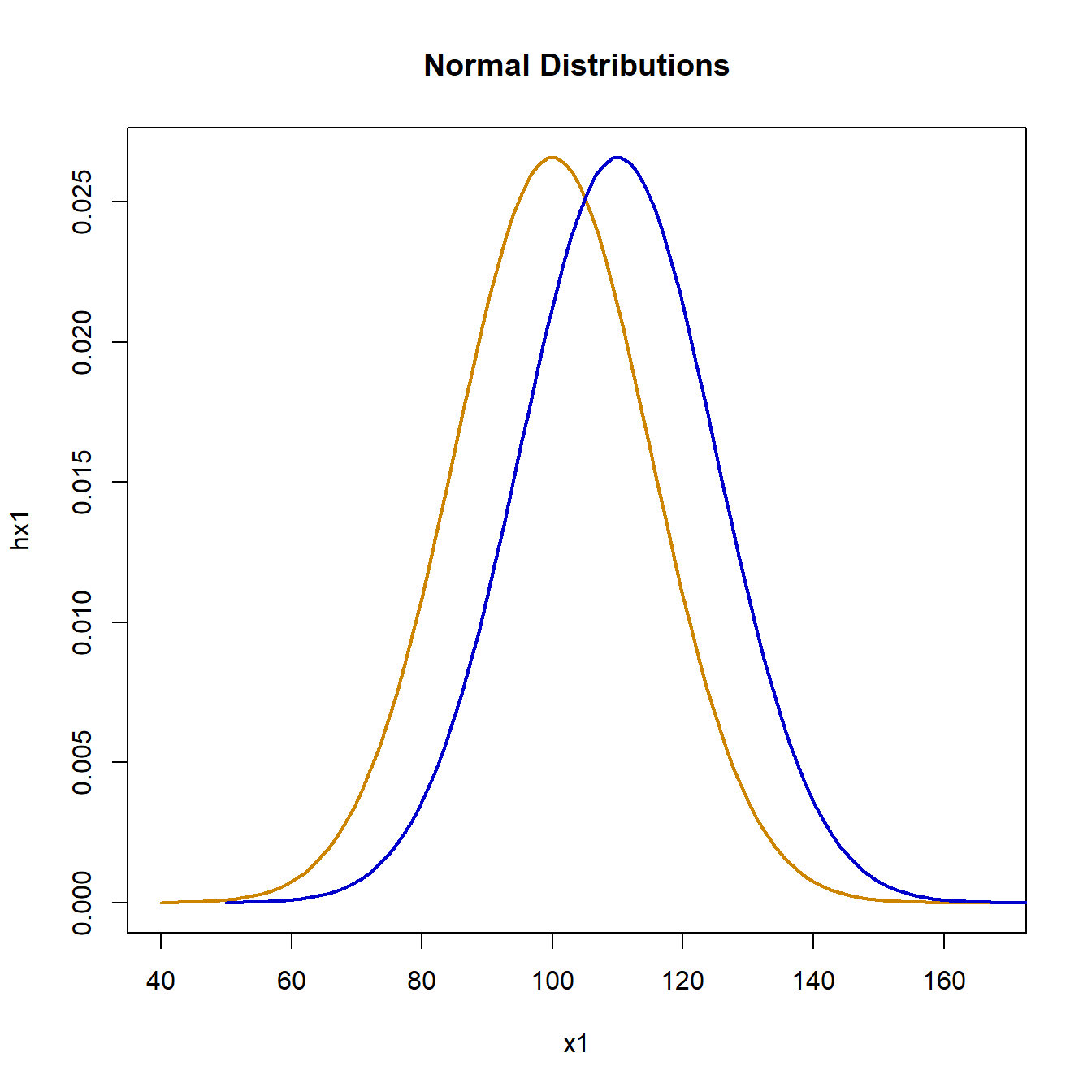
Normal Distribution

The first simulation will be conducted using normally distributed data.

set.seed(1)
mn1 <- 100
mn2 <- 110
stdev <- 15

x1 <- seq(-4, 4.5, length = 100)*stdev + mn1
x2 <- seq(-4, 4.5, length = 100)*stdev + mn2
hx1 <- dnorm(x1, mn1, stdev)
hx2 <- dnorm(x2, mn2, stdev)
plot(x1, hx1, type = "l", lwd = 2, col = "orange3", main = "Normal Distributions")
lines(x2, hx2, lwd = 2, col = "blue3")

Simulating the null hypothesis using normally distributed data for both groups drawn from the same distribution, gives the following:

nsim1 <- replicate(1000, t.test(rnorm(36, mn1, stdev),
                                rnorm(36, mn1, stdev),
                                var.equal = TRUE),
                   simplify = FALSE)
table(sapply(nsim1, "[[", "p.value") < 0.05)

## 
## FALSE  TRUE 
##   945    55

Out of 1,000 simulations, the test rejected the null hypothesis 55 times, close to the expected number of 50 based on the 5% significance level. Next, we simulate the alternative hypothesis using data drawn from different distributions:

nsim2 <- replicate(1000, t.test(rnorm(36, mn1, stdev),
                                rnorm(36, mn2, stdev),
                                var.equal = TRUE),
                   simplify = FALSE)
table(sapply(nsim2, "[[", "p.value") < 0.05)

## 
## FALSE  TRUE 
##   203   797

The test rejected the null hypothesis 797 times in 1,000 simulations, close to the expected 80% based on the power of the test.

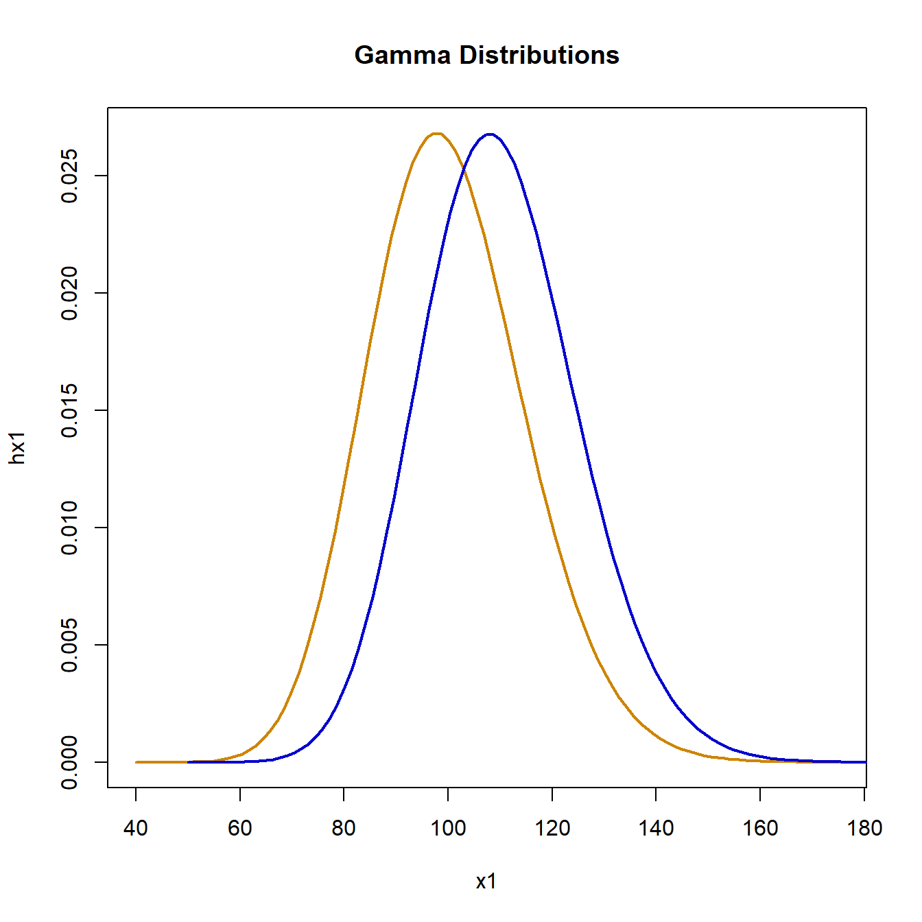
Gamma Distribution

The next set of simulations use data from a gamma distribution. The shape and scale parameters for a gamma distribution can be estimated using the method of moments:

gamma_mom <- function(mean, sd){
  if (mean > 0){
      theta <- sd^2/mean
      kappa <- mean/theta
  } else{
      stop("Mean must be positive")
  }
  return(list(kappa = kappa, theta = theta))
}

# Get parameters for gamma plot
mn1 <- 100
stdev <- 15
g1 <- gamma_mom(mn1, stdev)
mn2 <- 110
g2 <- gamma_mom(mn2, stdev)

# Plot of gamma distributions
x1 <- seq(-4, 5, length = 100)*stdev + mn1
x2 <- seq(-4, 5, length = 100)*stdev + mn2
hx1 <- dgamma(x1, shape = g1$kappa, scale = g1$theta)
hx2 <- dgamma(x2, shape = g2$kappa, scale = g2$theta)
plot(
  x1, hx1, type = "l", lwd = 2, col = "orange3",
  main = "Gamma Distributions"
)
lines(x2, hx2, lwd = 2, col = "blue3")

Drawing both sample groups from a gamma distribution with mean 100 and standard deviation 15, we simulate the null hypothesis as follows:

gsim1 <- replicate(1000, t.test(rgamma(n = 36, shape = g1$kappa, scale = g1$theta),
                                rgamma(n = 36, shape = g1$kappa, scale = g1$theta),
                                var.equal = TRUE),
                   simplify = FALSE)
table(sapply(gsim1, "[[", "p.value") < 0.05)

## 
## FALSE  TRUE 
##   953    47

The null hypothesis was rejected 47 times, close to the expected number of 50 based on the 5% significance level. Next, we simulate the alternative hypothesis using data drawn from different distributions:

gsim2 <- replicate(1000, t.test(rgamma(n = 36, shape = g1$kappa, scale = g1$theta),
                                rgamma(n = 36, shape = g2$kappa, scale = g2$theta),
                                var.equal = TRUE),
                   simplify = FALSE)
table(sapply(gsim2, "[[", "p.value") < 0.05)

## 
## FALSE  TRUE 
##   184   816

The test rejected the null hypothesis 816 times in 1,000 simulations, as expected.

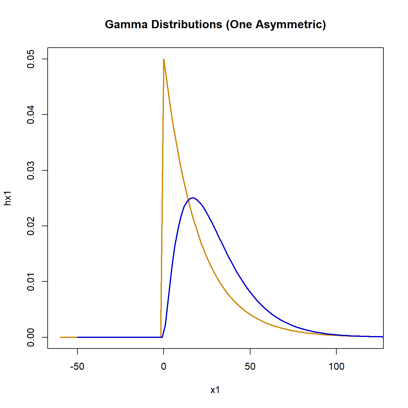
When the gamma distribution has a large shape parameter, the distribution is approximately normal, though slightly asymmetric. To increase the asymmetry, we’ll use gamma distributions with a smaller mean.

# Parameters will gamma distribution
mn3 <- 20
stdev <- 20
g3 <- gamma_mom(mn3, stdev)
mn4 <- 30
g4 <- gamma_mom(mn4, stdev)

# Plot of gamma distributions
x1 <- seq(-4, 5, length = 100)*stdev + mn3
x2 <- seq(-4, 5, length = 100)*stdev + mn4
hx1 <- dgamma(x1, shape = g3$kappa, scale = g3$theta)
hx2 <- dgamma(x2, shape = g4$kappa, scale = g4$theta)
plot(
  x1, hx1, type = "l", lwd = 2, col = "orange3",
  main = "Gamma Distributions (One Asymmetric)"
)
lines(x2, hx2, lwd = 2, col = "blue3")

Simulating the null hypothesis using data for both groups drawn from the same gamma distribution with mean 20 and standard deviation 20, gives the following:

gsim3 <- replicate(1000, t.test(rgamma(n = 36, shape = g3$kappa, scale = g3$theta),
                                rgamma(n = 36, shape = g3$kappa, scale = g3$theta),
                                var.equal = TRUE),
                   simplify = FALSE)
table(sapply(gsim3, "[[", "p.value") < 0.05)

## 
## FALSE  TRUE 
##   956    44

The null hypothesis was rejected 44 times out of 1,000 simulations, marginally lower than expected. For the alternative hypothesis simulation, the second distribution will have a mean of 30 and standard deviation 20, resulting in a long right tail.

gsim4 <- replicate(1000, t.test(rgamma(n = 36, shape = g3$kappa, scale = g3$theta),
                                rgamma(n = 36, shape = g4$kappa, scale = g4$theta),
                                var.equal = TRUE),
                   simplify = FALSE)
table(sapply(gsim4, "[[", "p.value") < 0.05)

## 
## FALSE  TRUE 
##   423   577

This time the null hypothesis was rejected 577 times in 1,000 simulations, a serious departure from the 80% expected for normally distributed data.

Uniform Distribution

The next set of simulations use data from an uniform distribution.

# Parameters
mn1 <- 100
mn2 <- 110
stdev <- 15

# Plot of uniform distributions
x1 <- seq(-3, 3, length = 100)*stdev + mn1
x2 <- seq(-3, 3, length = 100)*stdev + mn2
hx1 <- dunif(x1, min = 74, max = 126)
hx2 <- dunif(x2, min = 84, max = 136)
plot(x1, hx1, type = "l", lwd = 2, col = "orange3", main = "Uniform Distributions")
lines(x2, hx2, lwd = 2, col = "blue3")

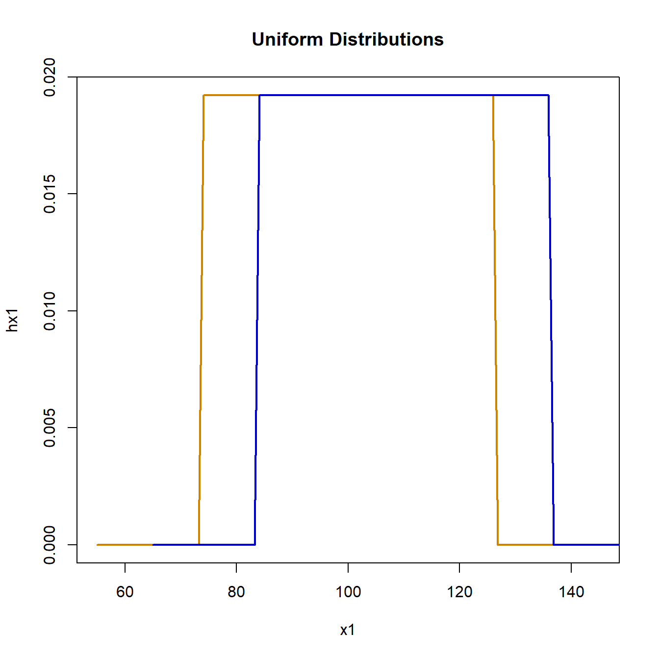
Using random samples from the interval [74, 126], representing a uniform distribution with mean 100 and standard deviation 15, simulation of the null hypothesis is:

usim1 <- replicate(1000, t.test(runif(n = 36, min = 74, max = 126),
                                runif(n = 36, min = 74, max = 126),
                                var.equal = TRUE),
                   simplify = FALSE)
table(sapply(usim1, "[[", "p.value") < 0.05)

## 
## FALSE  TRUE 
##   945    55

The test rejected the null hypothesis 55 times, close to the expected number of 50 based on the 5% significance level. Moving the second distribution over by 10 by drawing from the interval [84, 136], the alternative hypothesis simulation is:

usim2 <- replicate(1000, t.test(runif(n = 36, min = 74, max = 126),
                                runif(n = 36, min = 84, max = 136),
                                var.equal = TRUE),
                   simplify = FALSE)
table(sapply(usim2, "[[", "p.value") < 0.05)

## 
## FALSE  TRUE 
##   196   804

The test rejected the null hypothesis 804 times out of 1,000 simulations, marginally lower than expected, but not remarkable.

Student-t Distribution

Finally, we simulate from a Student-t distribution, a symmetric distribution, heavier in the tails than the normal distribution.

# Load library
library(metRology)

## 
## Attaching package: 'metRology'

## The following objects are masked from 'package:base':
## 
##     cbind, rbind

# Parameters
mn1 <- 100
mn2 <- 110
stdev <- 15
df1 <- 6

# Plot of t distributions with df = 6
x1 <- seq(-5.2, 5.2, length = 100)*stdev + mn1
x2 <- seq(-5.2, 5.2, length = 100)*stdev + mn2
hx1 <- dt.scaled(x1, df = df1, mean = mn1, sd = stdev)
hx2 <- dt.scaled(x2, df = df1, mean = mn2, sd = stdev)
plot(
  x1, hx1, type = "l", lwd = 2, col = "orange3",
  main = "Scaled t Distributions (df = 6)"
)
lines(x2, hx2, lwd = 2, col = "blue3")

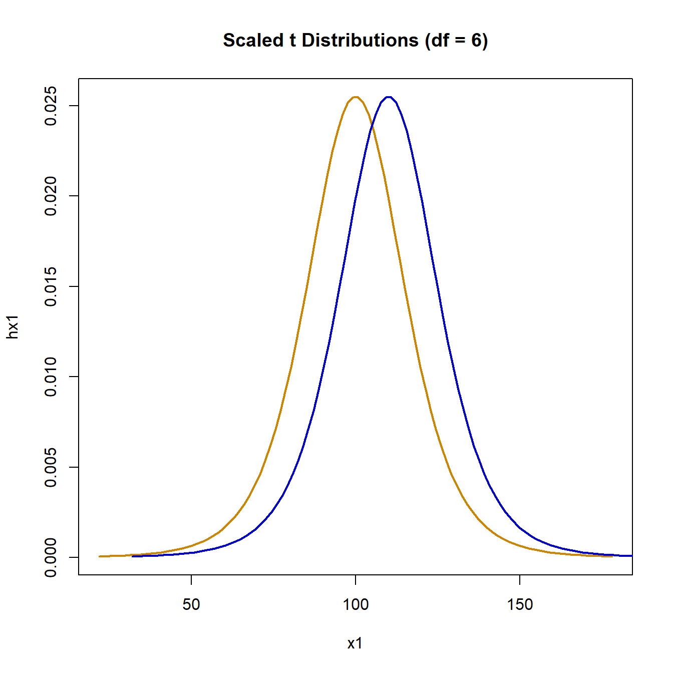
Simulating the null hypothesis using data for both groups drawn from the same t-distribution with degrees of freedom (df) of 6 gives:

tsim1 <- replicate(1000, t.test(rt.scaled(36, df = df1, mean = mn1, sd = stdev),
                                rt.scaled(36, df = df1, mean = mn1, sd = stdev),
                                var.equal = TRUE),
                   simplify = FALSE)
table(sapply(tsim1, "[[", "p.value") < 0.05)

## 
## FALSE  TRUE 
##   958    42

When both groups come from the same t distribution, the null hypothesis is rejected 42 times. When the second distribution is shifter to have mean 110, the simulation gives:

tsim2 <- replicate(1000, t.test(rt.scaled(36, df = df1, mean = mn1, sd = stdev),
                                rt.scaled(36, df = df1, mean = mn2, sd = stdev),
                                var.equal = TRUE),
                   simplify = FALSE)
table(sapply(tsim2, "[[", "p.value") < 0.05)

## 
## FALSE  TRUE 
##   360   640

The null hypothesis is rejected 640 times out of 1,000 simulations. This is significantly lower than the expected 80%. A t-distribution with 6 degrees of freedom has a heavy tail compared to a normal. Using a heavier tail by using 3 degrees of freedom, the null hypothesis simulation is:

df2 <- 3
tsim3 <- replicate(1000, t.test(rt.scaled(36, df = df2, mean = mn1, sd = stdev),
                                rt.scaled(36, df = df2, mean = mn1, sd = stdev),
                                var.equal = TRUE),
                   simplify = FALSE)
table(sapply(tsim3, "[[", "p.value") < 0.05)

## 
## FALSE  TRUE 
##   954    46

The test rejected the null hypothesis 46 times, marginally lower than expected. When the second distribution is shifter to have mean 110, the alternate hypothesis simulation with df of 3 is:

tsim4 <- replicate(1000, t.test(rt.scaled(36, df = df2, mean = mn1, sd = stdev),
                                rt.scaled(36, df = df2, mean = mn2, sd = stdev),
                                var.equal = TRUE),
                   simplify = FALSE)
table(sapply(tsim4, "[[", "p.value") < 0.05)

## 
## FALSE  TRUE 
##   562   438

Shifting the second distribution over to have mean 110, the null hypothesis is rejected 438 times out of 1,000, significantly less than 80%, which is expected if the data were normally distributed.

Conclusion

These examples show that the two-sample t-test can be used for data with a moderate tailed, symmetric distribution. When the data come from a heavy tailed distribution, even one that is symmetric, the two-sample t-test may not perform as designed. Under these conditions, it would be better to use a nonparametric test, such as the WRS test, the randomization test, or the Kolmogorov-Smirnov test.